The basic principle of the radar is to send a pulse (a flash) of radio waves (invisible light) wait and receive back scattered radiation (echo or reflexion). Distance of the reflecting object is derived from the duration of the delay between transmit and receive.
In order to illustrate the howtos, I will take as an example the image of the Beaugency town image in the image gallery. This is a X-band (10GHz frequency) image with a resolution of 60cm and full polarimetric measure. This is a typical average SAR image (I must emphasise it is definitely not ONERA's state of the art, it is an "easy made" but illustrative image). Illustrations and animations below are (of course) only low resolution thumbnail sized images, if you want to see the full resolution image (for a single integration) click here (beware it weights 175kB)
The delay is twice the distance divided by the velocity of light. Twice because the light travels forth and back, I insist on the radar being an active sensor: Like an usual camera with a flash, it illuminates the scene it makes an image of. To give an order of magnitude, if a radar observes a scene at a 5km distance, delay between transmit and receive is about 33µs (33 millionth of a second). Generally airborne radars wait until echo is received to transmit a new pulse, thus the pulse repetition frequency (PRF) in our example is below 30kHz (30,000 pulse per second). In space-borne cases, corresponding pulse repetition rates would be too low (see next chapter to know why) and generally between two pulse transmission, they receive echos from a much earlier pulse (i.e. they have always a few tens of pulses "in flight") but it makes no problem to know which echo correspond to which pulse because as seen from space, Earth surface (or any other planet one) is very smooth.
We use the generic term "light" as an equivalent to "electromagnetic wave", basically radio-waves are lower frequency (flatter tune) of the same physical phenomenon as visible light. To give ideas, the frequency of the X-band radio-waves is 1/60000 of that of visible light (or 16 octaves below). Typical radar frequencies range from a few hundred of mega-Hertz - 100,000,000 cycles per second up to a hundred of Giga--Hertz - 100,000,000,000 cycles per second (compared to 600,000,000,000,000 cycles per second for yellow light).
Velocity of radio-waves in the lower atmosphere is very close to the velocity of light in vacuum (299,792,458 m/s), radio-wave scientists express the deviation from the vacuum as "co-index" which is the deviation in ppm (parts per million). Standard atmosphere co-index is about 300ppm at sea level, real value fluctuates mostly with air moisture. Its impact on radar processing is negligible except in very high resolution case and for long range interferometry applications.
One crucial concept is the concept of resolving power: If we want to see details separated in range of say d=60cm, we should be separating echoes separated by no more than 2×d/c (where c denotes the velocity of light), which in our example is 4ns (four billionth of a second). We shall see later that this is a big deal...
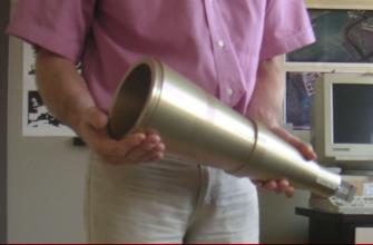
The real antenna is directional (unlike your mobile phone antenna), it emits radio-waves into a beam whose width is about 10° (very similar to that of a torch lamp). In practise, lower frequency means heavier, bigger and less directional antennae. Since our P-band (lowest frequency available at ONERA) antenna weights 80kg, I choose to hold much smaller Ku-band antenna (very similar to the one used for our example image) on the picture below. Radio-waves are generated at the small end of the cone, and radiated from the larger end.
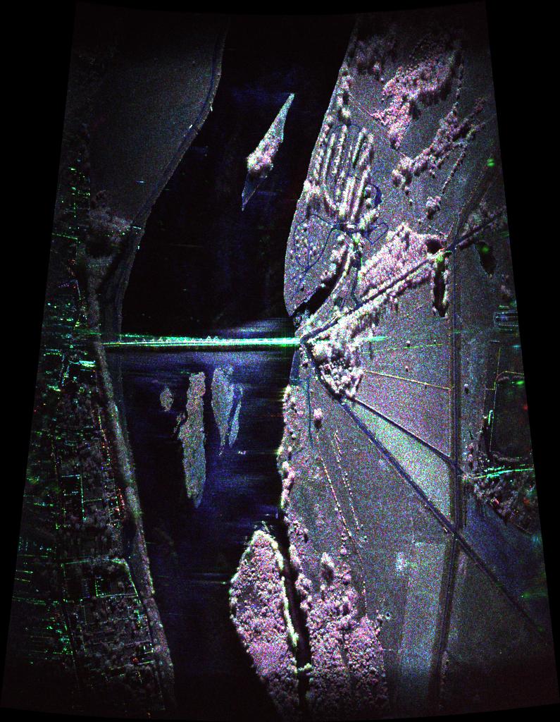
Hence assuming, we are able to record the echoes received with an accuracy of 4ns, we shall obtain with a single pulse an image such as this one:
The little grey dash at the left side is the aircraft position, (it flies toward the top) radar antenna looks through the right side door, and the illuminated area is about 1000×800m. More visually, the transmitted pulse propagates as an inflating sphere from the antenna (it inflates at light velocity, hence all this occurs within microseconds):
As the pulses reaches the ground it bounces on it in a relatively non-directional way (from a physical viewpoint, it diffract almost isotropically when roughness of the surface is important at the wavelength scale, here at the 3cm wavelength, landscape features -perhaps a few metallic walls excepted- are rough enough for the isotropic scattering called Lambert's law to apply). Thus only a minute fraction of the transmitted power is scattered back precisely into the 10cm wide aperture of the antenna horn. In the following image it is only the part exactly in front of the grey dash symbol for the antenna that shall be received. The bright white arc in the middle on the image is the strong reflection on the bridge propagating back towards the antenna:
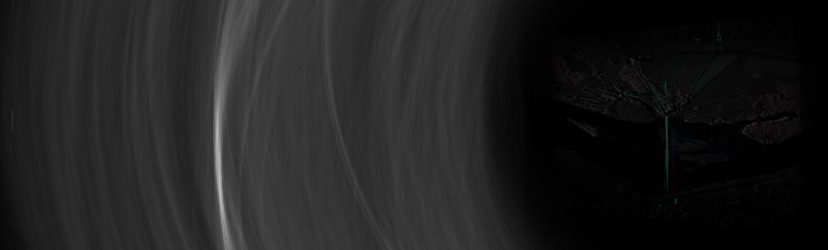
In fact most transmitted wave goes away, and things are even worse if surface is smooth, in that case the surface behave as a mirror and the light is reflected to the sky on the right hand side of the picture. This explains why smooth surface (such as the water in the river) appears darker than the rough surfaces (as forest or urban areas). It worth noting that turbulence on the water flow after the bridge (on the right of it, water flows from left to right) causes a lighter shade! On the image we can also notice that the overall length of the echo is twice the length of the illuminated area, this is again a consequence on the fact that light has to travel two ways forth and back. Dynamical aspect of the back-scattering phenomenon is visually interesting, click here to see a (550kB) film showing it (if it fails try this link, beware, this is an oddly shaped film 914×276 you might have to disable "aspect ratio" function of your visualiser application, I also suggest to set the "original size" option)
The fact that the received energy is extremely small compared to emitted one explains why most radars transmit and receive alternatively (the so called "continuous wave radars" are only used for very short range cheap applications). It also explains why long range radars require expensive low noise amplifiers on receive and huge transmitting power (to my knowledge the few nuclear power plants launched in space were for powering Earth observing radar Russian satellites)
Note, that the simulation above is only conceptual, real waves interfere and a more realistic image should be speckled as the full resolution image is. This is due to the fact that radar emitted light is coherent (in fact a radar transmitter behaves more like a laser than like a torch lamp). If you have a laser pointer, you certainly already noticed that the red spot is produces on a projection screen has this typical speckle (grainy) aspect. I discarded speckle in the simulation, because it blurs the interesting effects and it increases a lot the file size of the film (noise is hard to compress).
In order to be able to resolve 60cm in range, I mentioned that we should separate echos delayed by 4ns. In the previous scheme, it means that the pulse duration is smaller than 4ns (otherwise, the two echoes overlap). The average power of the ONERA radar used for our example was 100W (the power of a lamp bulb, or 1/10th of the power of an hairdryer), since pulses are spaced by 62.5µs the transmitter peak power should be 1.56MW (when it amplifies the pulse). Needless to say that an high fidelity mega-Watt amplifier, if it exists, should be extremely expensive, and probably too heavy to put on-board a plane (don't even think of launch it into orbit!). Thanks to Jean-Baptist Joseph Fourier (1768-1830), there is a solution called "pulse synthesis" or "pulse compression" (If you heard about mega-joule lasers, they function on a very similar way).
Now, what is the principle of the synthetic pulse. The genius idea due to Fourier, is that periodic functions can be decomposed as a sum of sinusoid of frequency multiple of that of the original function (these multiple are called the harmonics of the frequency of the function). He also gave mathematical formulae to compute the amplitude and phase (shift along time) of the sinusoidal component. The idea generalises, and decomposition of an arbitrary signal into sinusoid provides what is called the spectrum for the signal. It was named the spectrum because it is similar to the process of decomposing white light with a prism and making a rainbow-like spectrum spreading the higher frequencies on the blue side and the lower frequencies on the red side. Several early computer scientists (History retained the names of Gordon Sande, J.W. Cooley and Z.W. Tukey) found efficient algorithms for computing the decomposition, thereafter called fast Fourier transform (FFT). The second interesting point is the shape of the spectrum of a perfect pulse: it is perfectly constant! And in fact real pulses have a flat spectrum of width that is inversely proportional to the pulse-width. Thus, if one take a pulse, separate its frequency components and successively transmit them (i.e delay each component proportionally to its frequency) the pulse power will be spread in time evenly, and the peak power can be reasonable even for initially very short pulses.
In fact, the real design of a radar is even trickier than that: The real short pulse is never generated in the circuits, instead, the resulting spread impulsion is calculated on a computer and loaded before flight into radar memories. On transmit, the radar electronics scans this memory and playback the corresponding signal. The signal has a relatively simple expression called "chirp" (because audio waves of the same shape sound like bird chirps click here to hear an audio transposition of our example waveform. Honestly it does not really sound as birds, I tried to transpose another waveform click here to hear an audio transposition of our P-band (lower frequency, foliage/ground penetrating) waveform). The formula is:
sin(ft+ßt²)
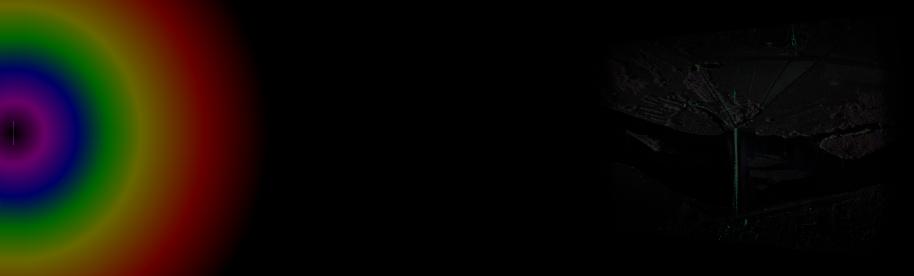
Just to illustrate the principle, here is what correspond to the transmitting of a synthetic pulse (modulated as a linear chirp) where the signal frequency is coded with increasing frequency coloured from red to blue (just like in visible light). In our example red corresponds to 9.45GHz and blue corresponds to 9.69GHz, duration of the transmit is 26µs (thus the instantaneous peak power is lowered down to 250W which is reasonable to laboratory grade equipment!)
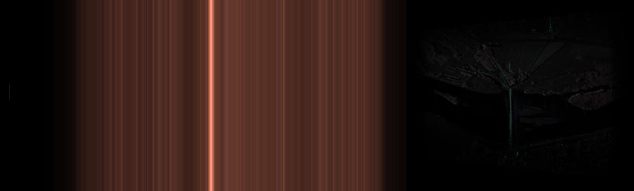
the back-scattered echo is also spread:

Note that back-scatter length is now twice the illuminated area length plus the chirp length. Echo is mostly colourless in the middle, the strong echo from the bridge appears as a subtle rainbow-like hue zone in the middle of the echo, note that the signal energy is more evenly smoothed. The dynamics of the scattering process is less visually striking than with real pulse click here to see a 940kB film showing it (if it fails try this link).
The recovery of the real pulse-like echo requires to delay the successive frequencies in the echo by an amount opposite to the one introduced before transmit. This operation is (at least partially) done by calculators after digitising of the signal. This computation yields a "range compressed" echo similar to the one that would have been obtained with a real 4ns wide pulse:
click here to see a 466kB film illustrating the pulse compression process (if it fails try this link).
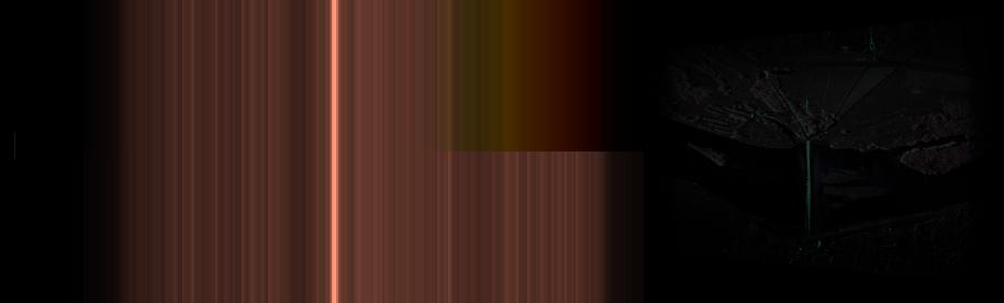
The above images are computed assuming that the whole echo of the landscape is actually recorded and processed. It is common however that the pulse recording is truncated (especially at the far range end when the incidence angle is grazing). In that case the end of the range profil is reconstructed with only a part of the bandwidth (hence appears colored and dimmed in the following illustration) but more important is the fact that the reduced bandwidth available there implies a coarser resolution. This is this phenomenon that occured in the far range (right side) of the Paris SAR image shown in the gallery. Illustration of this phenomenon on our example data is given in the top half of the following image (the lower half gives the untruncated signal after recompression for comparison):
click here to see a 453kB film illustrating the pulse compression process with and without signal truncature. (if it fails try this link).
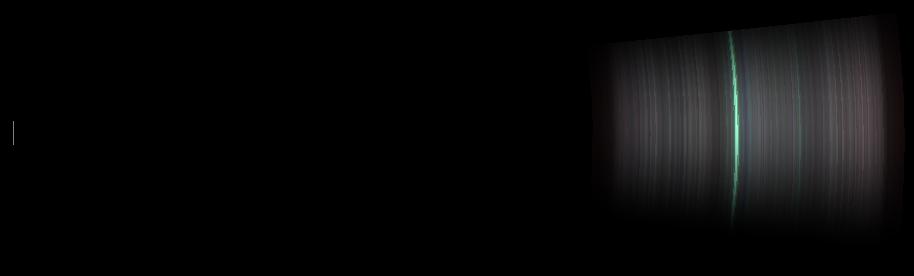
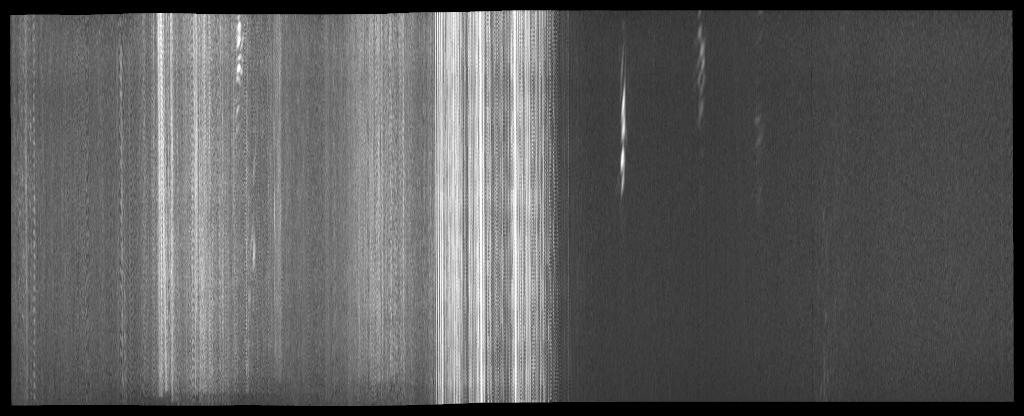
To show the lower dynamical range obtained with synthetic pulse, here is an image of the raw signal from our example. Columns correspond to pulses (times goes from top down), and successive pulses acquired as the aircraft proceeds are aligned left to right. Signal is even flatter (along the vertical axis) than in the above simulations because an electronic preprocessing called deramping was applied:
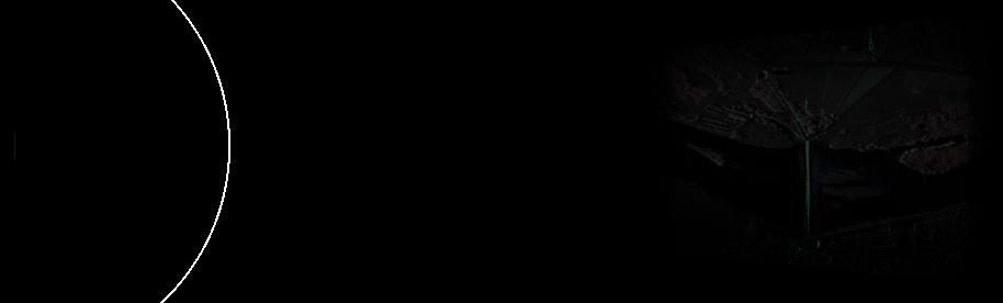
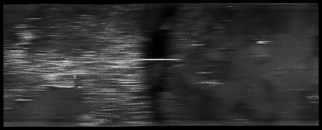
At this point in the procession, we only accurately solve for the distance of features on the landscape, but this is not enough because, as I mentioned above, the real antenna has a beam-width (antenna pattern) 10° wide, hence even if we steer the antenna to scan the landscape, we obtain an image with 60cm range resolution but merely 500m resolution on the steering direction. For example, that is the image one gets when the aircraft motion is used to scan the ground (it the so called push-broom mode of imaging) The image is rotated 90° clockwise with respect to the previous images because computer screens are wider than taller (there is another reason: Our SAR handling system always put the radar on the top of the image, because depth perception on the landscape is correct only if lighting comes from the top):
click here to see a 688kB film showing the acquisition process (if it fails try this link) As radar wouldn't be very interesting if only such images were produced, synthetic aperture is used in order to improve dramatically the cross-range resolution this is explained in the next chapter