Details on Fourier transform

The Fourier decomposition:

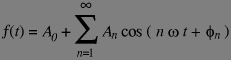
The idea of the Fourier transform, initially came from study of the periodic signals -namely the sound of an instrument single note- which analysed by a set of accoustic resonators showed that a given note was a mixture of the sinusoidal wave of a frequency corresponding to the perceived pitch of the note (what was denoted as the fundamental frequency) and sinusoid waves of frequencies multiples of that of the fundamental (that were denoted as the harmonics of the fundamental frequency). The difference in timbre between the same note played by distinct instruments corresponding to different relative levels between the fundamental and the harmonics. Joseph Fourier proved mathematically that (under technical conditions -namely is absolute integrability- not restrictive in practice for physicists) any periodic signal can be decomposed in a unique manner in a sum of sinusoids of frequency multiple of the signal frequency (denoted omega in the formula below):

In the above formula, the A coefficients are the amplitude of each harmonics and phi terms are their phases. It is also possible to change from the representation with amplitudes and phases to a sinus+cosinus representation, such as:

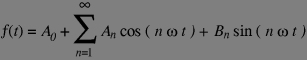
This representation is not the most convenient, especially for our use in which we shall translate frequencies, in that it does not make any difference between positive and negative frequencies. Indeed, on the circle drawn above changing omega to its opposite does not change the cosinus. For simplifying the notations and the algebraic manipulations, the complex numbers are used instead of real ones.

Using complex number, we can express a function of period T (or frequency F) as:

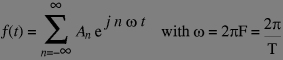
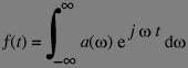
The A coefficients are complex numbers (if the function f is real valued, they have the property that A_-n and A_n are conjugate complexes). In fact, the above definition has been generalised to non periodic functions as well, and restricted to sampled signals (i.e. sequences of values instead of function of a real value). Sampled signals are also called discrete time signals. If the signal f is non periodic, its Fourier transformation is not made of only multiple of the fundamental frequency (since there is no such a thing) but from all the possible frequencies. The complex amplitude coefficients becomes a function defined for all real value for the frequency and the "sum indexed by the real number" is defined as an integral:

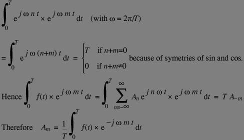
The use of sinuoids for decomposing a signal is interesting for two reasons: First the function set is sufficient for producing by linear composition any (reasonable) periodic function (as I mentioned above) but also these functions are mutually orthogonal (see below) which means that the Fourier decomposition is easy to compute. By orthogonality, we mean that the scalar product of two functions is zero. You know the definition of the scalar product in the 2D space [x₁,y₁].[x₂,y₂] = x₁×x₂ +y₁×y₂ and as you may remember, the two vectors [x₁,y₁] and [x₂,y₂] are orthogonal if their scalar product in zero. Indeed, this generalises to any dimensions of space, even infinite (infinite series and real valued functions for example):

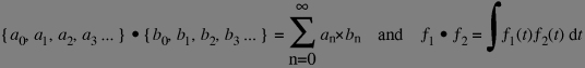
The integral being taken on the interval in which the functions are orthogonal (the fundamental period in our case). The orthogonality gives a simple way to compute the Fourier transform (FT in short):

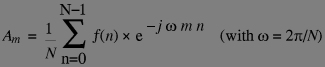
For using the FT in computers, we use it on sampled periodic signals (aperiodic signals are processed as padding them with zero to a period larger than their length, and used as if there where periodic). If you have a period of N samples, clearly the N^th harmonic of the fundamental (1/N) frequency is zero -the signal phase rotates one full turn, hence it does not change-. The formula for the discrete Fourier transform can be obtained by the same derivation:

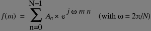
Note the relative similarity of the Fourier Transform computation formula above, and that of the signal using the Fourier coefficients below (remember there are only N-1 distinct harmonics the N^th = O^th is the constant 1 signal) that is also called the "inverse" Fourier transform:

As define above, the computation of an FT or an inverse FT (it is similar, but to the 1/N factor and the exponential conjugate), for all N values of m requires N² multiplications and additions of complex numbers -assuming that the exponential functions for the n,m values are tabulated (the matrix of these values is called the kernel of the N-point FT)-. This may seem not very costly (in terms of computer power requirement), but the computation of an image as our example image requires (for 800 lines of the image) 6000 FTs with N=4000 and 8000 FTs with N=2000, which makes a number of basic complex add and multiply (MAC) operations (1 MAC = 3 flop) of 128 bilion (384 Giga-flop). Even on todays computers, this is quite a deal. In fact, in the early 60's, many computer scientists devised fast algorithms based on the following principle: If you know the FT (say F and G) of two signals say A and B of length N, it is easy to compute the FT of the signals of the signals obtained by interleaving the signals A and B to respectively even and odd samples of a signal of length 2N (each sample is the linear combination of only two samples of the F and G spectra). The precise formula requires two properties described below (the Dirac comb transform and the delay-phase relationship) but already you can figure that if your sample number N is a power of two (say 2^k) The number of MAC's needed to obtain the N sample spectrum from the 2 N/2 sample spectra is 2N MACs, each of the 2 N/2 spectra can be computed from the 4 N/4 long spectra with 2N MACs either, and so on up to the 1 sample FT which is no change at all! Hence the total N point Fourier transform requires only 2Nk MACs (or 2Nlog₂(N) MACs). This is the Fast Fourier Transform (or FFT in short) ubiquitous in signal processing.

From the definitions of FT (either dicrete or continuous, periodic and aperiodic cases) we can derive crucial properties:

• Linearity: The FT of the sum of two signals is the sum of the FT of each signals: FT(f+g) = FT(f) + FT(g). The FT of a signal multiplied by a given complex number is obtained by multiplying by this number the FT of the signal: FT(z×f) = z×FT(f) (z being a constant)
• The FT of a signal delayed is the product of the FT of the signal with a pure frequency proportional to the delay:
• If a signal of period T is sampled on N points (hence samples are spaced by T/N or the frequency of sampling is N/T) its FT has N frequency samples spaced by 1/T.
• The frequency ±N/2 (note the indeterminacy over sign) is the highest frequency representable (corresponding to the sequence +1,-1,+1,-1,+1,-1 ...) This frequency is called the Nyquist frequency: if you sample a real valued signal of bandwidth ±B with a sampling frequency below 2B, frequencies above +N/2 will be mixed (irreversibly) with frequencies above -N/2 and conversely, thus your spectrum will be wrapped up (it is also called aliasing).

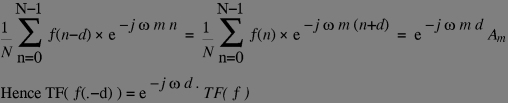
FT of some particular signal worth to be known (if you know college-grade calculus, you may compute these formally): A perfect pulse at zero (the sequence 1,0,0,0,0) correspond to a constant spectrum. A perfect pulse at a nonzero position correspond to a pure frequency (remember the delayed FT formula above?), A Dirac comb of period N/M (i.e. M ones evenly spaced by zeroes) correspond to a Dirac comb of period M/N (i.e. N/M ones evenly spaced by zeroes). A rectangle function of width 2W (i.e. a function value of 1 between -W and +W and zero elsewhere) is (approximatively in dicrete case, exactely in aperiodic continuous case) 2Wsinc(2piWF).

The last decisive FT property is the convolution theorem. First, we must define the convolution as the operation which takes two signals F and G produces a results F*G defined as follow: for each sample F_n of F, add to the result the sequence G shifted by n samples and multiplied the constant F_n. This operation requires N2 complex multiplications and additions and the "slow" FT, but the convolution theorem states that: FT(F*G)=FT(F)×FT(G) i.e. the samples of the FT of F*G are the product of the corresponding samples of FT(F) and FT(G) respectively. Hence using FFT's, the most efficient computation for F*G is to compute FT-1(FT(F)×FT(G)). It also provide a way to perform a deconvolution: if you measured F*G with some known function G (G can be for example a focus or motion blur function) you can retrieve the unknown signal F by FT-1(FT(F*G)÷FT(G)) -provided the spectrum of G (FT(G)) does not vanish on the support of the spectrum of the unknown F).