22 Sept. 2021
Geometry of the Branching Point
I was reading Samir Okasha's Agent and Gaols in Evolution (2018) for our evolution and optimality workgroup and a passage describing an evolutionary branching point gave me pause:
"In this way natural selection leads the population to converge to x^* from nearby points, despite x^∗ being a minimum, not a maximum, of the fitness function. The fact that natural selection can lead to fitness minimization is rather counter-intuitive, conflicting with our everyday understanding of how natural selection is supposed to work."
— Okasha (2018) pp. 111-112
This strikes me as odd. Intuitively, I would agree that the branching point is indeed a minimum for the invasion fitness with respect to the mutant trait, but it's also a saddle (or "minmax") point when considering the invasion fitness surface. In what extent is it a "convergence toward a minimum" really ?
I find this question interesting because it has real weight in the overarching debate any modeller face at some point: when and where can we consider that natural selection can be reduced to an optimisation process, climbing up an hill of fitness ?
I guess it's a good an excuse as another to have a look at the geometry of the branching point. This post assumes some familiarity with the concepts of adaptive dynamics (invasion fitness, pairwise invasibility plots…). If you need a refresher, you can read the very accessible hitchhiker guide by Brännström et al. (2013), the original article by Geritz et al. (1998) or my own tutorial.
Competition toy model
Ecology
Consider the following ecological model describing the dynamics of the population density (n_i) of several types of individuals:
\frac{d n_i}{dt} = n_i \left [ k(i) - \sum_{j=1}^N n_j d_u(i,j) \right ]
I took simple Gaussian-like forms for k and d: k(x) = e^{-x^2} and d_u(x,y) = e^{-[u(x-y)]^2}. The goal here is not to have a realistic ecology, but a simple model to investigate the geometry of the branching point.
Thus, k is optimal around a trait value of 0. Additionally, competition is symmetric, and always stronger between individuals with similar traits. The parameter u controls the specificity of the competition. Indeed, consider the competition between x and y: if u is high, x\mapsto d_u(x,y) is narrow around y, and decays quickly for values of x that are far away. Whereas if u is low, x\mapsto d_u(x,y) decreases slower.
Adaptive dynamics
If there are only two types in the population (a resident r and the mutant m), the system becomes:
\begin{cases} \frac{d n_r}{dt} = n_r ( k(r) - n_r d_u(r,r) - n_m d_u(r,m))\\ \frac{d n_m}{dt} = n_m ( k(m) - n_r d_u(m,r) - n_m d_u(m,m)) \end{cases}
When there is no mutant, n_m(0)=0 the equilibrium of the resident population is n_r^*=\frac{k(r)}{d_u(r,r)}. The invasion fitness of a mutant with trait m in a monomorphic resident population at equilibrium with trait r is given by:
\begin{align} s(r,m) &= \frac{1}{n_m}\frac{d n_m}{dt} \huge|_{n_r = n_r^*}\\ & = k(m) - k(r) \frac{d_u(r,m)}{d_u(r,r)} \end{align}
There is an evolutionary singular point around r=0. Regardless of the value of parameters, this singular point is convergence stable. Additionally, there's a "bifurcation" point in u=1: for values u<1, the evolutionary singular point x=0 is an Evolutionary stable strategy (ESS), while for u>1, the singular point is a branching point.
You can mouse over the u axis to change its value and see the consequence on the Pairwise Invasibility Plot. The grey areas represent positive value of s(r,m), while white represents negative values. Circles indicate evolutionary singular points (blue for ESS, orange for Branching points).
From a purely geometric point of view, the evolutionary singular point is always a saddle point of the invasion fitness surface (with two "valleys" in white and two "hills" in black). The nature of the singular point depend on the position of those hills and valleys relatively to the y-axis. Indeed, remember that if the population is at the singular point r=0 mutants can only appear on the vertical line (r=0, m \in \mathbb R). The singular point is an ESS if the mutants at the singular point fall in the valley (cannot invade, the point is evolutionarily stable), and a branching point if the mutants fall on the hill (can invade, the point is evolutionarily unstable).
Trait substitution Sequence
Now we look at a succession of mutations-invastion. Starting from a monomorphic population with trait r, a mutant trait value m is generated at each timestep (normally distributed around r) and it invade the population (i.e. replaces the resident) if and only if s(r,m)>0 (otherwise the population stays in r. This constitute the trait substitution sequence (TSS). (Note that we could take the approximation that the mutations are infinitesimal to recover the so-called "canonical equation" of adaptive dynamics).
You can click on the u axis to change its value and see the consequence on the Trait substitution sequence
In cases where the singular point is an ESS, the convergence of the TSS makes no doubt. If we look at the cross-section of the fitness landscape s(r,m) as a function of m, there is a hill and the population is neatly climbing it to the optimal value.
In the case of the branching point, though, the cross section ends up looking like an unstable bowl. While it seems like the population is moving toward the minimum point of this curve, it never really quite reach it. It's not really a march toward the minimum and more a kind of Penrose stairs where every step up (a mutant invading) somehow never amount to climbing in altitude (reaching a peak of the fitness landscape).
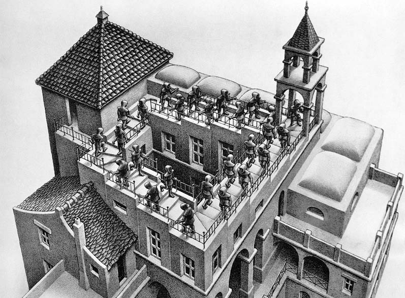
Ascending and Descending (1960), M. C. Escher (Detail). In this lithograph, Escher represents an example of Penrose stairs: despite always going up, the character ends up back in its initial position.
Here I limited myself to a situation where mutations are so rare that they appear sequentially. However the big insight of the adaptive branching theory is, of course, that if two mutant phenotypes appear in the population at the same time, they can be maintained and keep on diverging, but that's outside of the scope of this quick exploration.
On Optimisation
I read this article in the context of a work-group reviewing the "optimising" nature of Natural selection. While I think the branching point is a bad argument for fitness minimization, it certainly illustrates well the limits of fitness landscape metaphors.
Here there does not seem to be a fixed fitness landscape to climb, because any new mutant invading changes the selective environement and thus the shape of this landscape. Conversely, it does not mean that natural selection lead to fitness minimization as it is sometimes hastily claimed: every mutant-invasion step is going up in the landscape at the time of the mutation. It's just that on the long run, the landscape changes.
Birch (2016) do a pretty good review of the arguments for and against treating natural selection as a process of fitness maximisation. And the bottom line is that, so far, all arguments in favour of treating natural selection as an optimising process require that the environement be stable. As he puts it : "this may be the most we can expect from theory alone. After all theory alone cannot establish the long-run invariance of selective environements, or the long-run malleability of genetic arangements." (p716, emphasis is mine). I would tend to agree.
This is also why I tend to be wary of sweeping arguments that equate natural selection with an optimising process. And I think that, overall, approaches such as Formal Darwinism (Grafen, 2014) will not overcome the limits of theory outlined by Birch. Optimisation needs a somehow stable environement, but that cannot be the norm, if only because of eco-evolutionary feedbacks (Doulcier et al. 2021).
Overall, I don't think it's an insurmountable problem, and it does not mean that any field where the optimality of organisms is assumed (such as evolutionary ecology) lack theoretical grounding. It just allow that those assumptions should not be done carelessly, but always accompanied by a (not perfunctory) assumption of long-term stability of environmental effects. When those assumption do not hold though, interesting biology might occur.
References
- Brännström, Å., Johansson, J., & von Festenberg, N. (2013). The Hitchhiker’s Guide to Adaptive Dynamics. Games, 4, 304–328.
- Birch, J. (2016). Natural selection and the maximization of fitness: Natural selection and the maximization of fitness. Biological Reviews, 91(3), 712–727. https://doi.org/10.1111/brv.12190
- Doulcier, G., Takacs, P., & Bourrat, P. (2021). Taming fitness: Organism-environment interdependencies preclude long-term fitness forecasting. BioEssays, 43(1), 2000157. https://doi.org/10.1002/bies.202000157
- Geritz, S. A. H., Kisdi, E., Meszéna, G., & Metz, J. a. J. (1998). Evolutionarily singular strategies and the adaptive growth and branching of the evolutionary tree. Evolutionary Ecology, 12, 35–57.
- Grafen, A. (2014). The formal darwinism project in outline. Biology & Philosophy, 29(2), 155–174. https://doi.org/10.1007/s10539-013-9414-y
- Okasha, S. (2018). Agents and goals in evolution (First edition). Oxford: Oxford University Press.