This post presents modern mechanisms and techniques for training interpretable models, it continues the series on interpretable models (please refer to the neighboring posts: 1. Context and 3. Best practices). The motivation for the used nomenclature has been addressed in the previous post

Contents

1. Data visualization approaches. Having a strong understanding of a dataset is a first step toward validating, explaining, and trusting models.
2. White-box modeling techniques. Models with directly interpretable internal mechanics.
3. Model-agnostic techniques. These techniques generate explanations even for the most complex models using model visualizations, reason codes, global variable importance measures.
4. Approaches for testing and debugging ML models for fairness, stability, trustworthiness.

Some of these interpretability mechanisms has been known for years, many others came out with the recent research.

Data visualization approaches

Seeing and understanding data is important for interpretable machine learning: machine learning models represent data, so understanding the contents of that data helps set reasonable expectations for model behavior and output and choose the most appropriate model architecture.

Most real datasets have too many variables and rows and are difficult to see and understand. Even if plotting many dimensions is technically possible, it would often rather detracts us from (instead of enhancing) understanding of complex datasets. Two following visualization techniques help illustrate datasets’ structure in just two dimensions: 2D projections and network graphs.

Technique	2D projections	Correlation network graphs
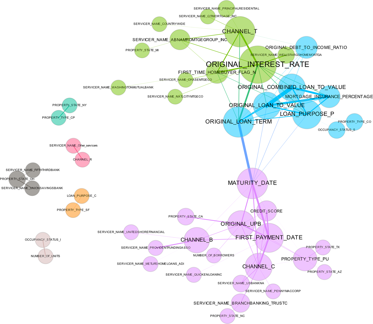
Description	Projecting rows of a dataset from a usually high-dimensional original space into a more visually understandable lower-dimensional space, ideally two or three dimensions. Some techniques to achieve this include principal components analysis (PCA), multidimensional scaling (MDS), t-distributed stochastic neighbor embedding (t-SNE), and autoencoder networks.	A correlation network graph is a 2D representation of the relationships (correlation) in a dataset. The authors create correlation graphs in which the nodes of the graph are the variables in a dataset and the edge weights (thickness) between the nodes are defined by the absolute values of their pairwise Pearson correlation. For visual simplicity, absolute weights below a certain threshold are not displayed, the node size is determined by a node’s number of connections (node degree), node color is determined by a graph community calculation, and node position is defined by a graph force field algorithm. The correlation graph allows us to see groups of correlated variables, identify irrelevant variables, and discover or verify important, complex relationships that machine learning models should incorporate, all in two dimensions.
Suggested usage	The key idea is to represent the rows of a dataset in a meaningful low-dimensional space. Datasets containing images, text, or even business data with many variables can be difficult to visualize as a whole. These projection techniques enable high-dimensional datasets to be projected into representative low-dimensional spaces and visualized using the trusty old scatter plot technique. A high-quality projection visualized in a scatter plot should exhibit key structural elements of a dataset, such as clusters, hierarchy, sparsity, and outliers. 2D projections are often used in fraud or anomaly detection to find outlying entities, like people, transactions, or computers, or unusual clusters of entities.	Correlation network graphs are especially powerful in text mining or topic modeling to see the relationships between entities and ideas. Traditional network graphs—a similar approach—are also popular for finding relationships between customers or products in transactional data and for use in fraud detection to find unusual interactions between entities like people or computers.
References	t-SNE, Multidimensional scaling, Reducing dimensionality with neural networks
OSS	Scikit-learn, R, H2O	Gephi, corr_graph
Global / local scope	Global and local. Can be used globally to see a coarser view of the entire dataset, or provide granular views of local portions of the dataset by panning, zooming, and drilldown.	Global and local. Can be used globally to see a coarser view of the entire dataset, or provide granular views of local portions of the dataset by panning, zooming, and drilling down.
Best-suited complexity	Any. 2D projections can help us understand very complex relationships in datasets and models.	Any, but becomes difficult to understand with more than several thousand variables.
Model-specific / agnostic	Model agnostic; visualizing complex datasets with many variables.	Model agnostic; visualizing complex datasets with many variables.
Trust, understanding	Projections add a degree of trust if they are used to confirm machine learning modeling results. For instance, if known hierarchies, classes, or clusters exist in training or test datasets and these structures are visible in 2D projections, it is possible to confirm that a machine learning model is labeling these structures correctly. A secondary check is to confirm that similar attributes of structures are projected relatively near one another and different attributes of structures are projected relatively far from one another. Consider a model used to classify or cluster marketing segments. It is reasonable to expect a machine learning model to label older, richer customers differently than younger, less affluent customers, and moreover to expect that these different groups should be relatively disjoint and compact in a projection, and relatively far from one another.	Correlation network graphs promote understanding by displaying important and complex relationships in a dataset. They can enhance trust in a model if variables with thick connections to the target are important variables in the model, and we would expect a model to learn that unconnected variables are not very important. Also, common sense relationships displayed in the correlation graph should be reflected in a trustworthy model.

A correlation network graph improves trust and understanding in ML models by displaying complex relationships between variables as edges and nodes in an undirected graph.

White-box modeling techniques

For high-stakes usecases, models might need to follow maximum transparency guidelines since inception, not to encounter fairness and security issues. Newer white-box modeling methods — XNN, monotonic GBM, scalable Bayesian rule lists — promote interpretability at minimal accuracy penalty (if any at all). Interpretable model will likely simplify debugging, explanation, and fairness auditing tasks as well.

The following techniques — decision trees, XNN-ANN, monotonic GBM, alternative regression (logistic, elastic net, quantile regression, GAMs), rule-based models, SLIMs — create transparent models well-suited for regulated industry and vital applications with extreme importance of interpretability.

Decision trees

Decision trees create a model that predicts the value of a target variable based on several input variables. Decision trees are directed graphs in which each interior node corresponds to an input variable. There are edges to child nodes for values of the input variable that creates the highest target purity in each child. Each terminal node or leaf node represents a value of the target variable given the values of the input variables represented by the path from the root to the leaf. These paths can be visualized or explained with simple if-then rules. In short, decision trees are data-derived flowcharts.

Suggested usage: Decision trees are great for training simple, transparent models on IID data— data where a unique customer, patient, product, or other entity is represented in each row. They are beneficial when the goal is to understand relationships between the input and target variable with “Boolean-like” logic. Decision trees can also be displayed graphically in a way that is easy for nonexperts to interpret.

References: L. Breiman et al., Classification and Regression Trees (Boca Raton, FL: CRC Press, 1984), Hastie et al., The Elements of Statistical Learning, Second Edition.

OSS: rpartscikit-learn (various functions)

Global or local scope: Global.

Best-suited complexity: Low to medium. Decision trees can be complex nonlinear nonmonotonic functions, but their accuracy is sometimes lower than more sophisticated models for complex
problems and large trees can be difficult to interpret.

Model specific or model agnostic: Model specific.

Trust and understanding: Increases trust and understanding because input to target mappings follows a decision structure that can be easily visualized, interpreted, and compared to domain knowledge and reasonable expectations.

XNN and ANN explanations

XNN, a new type of constrained artificial neural network, and new model-specific explanation techniques have recently made ANNs much more interpretable and explainable. Many of the breakthroughs in ANN explanation stem from derivatives of the trained ANN with respect to input variables. These derivatives disaggregate the trained ANN response function prediction into input variable contributions. Calculating these derivatives is much easier than it used to be due to the proliferation of deep learning toolkits such as Tensorflow.
Suggested usage: While most users will be familiar with the widespread use of ANNs in pattern recognition, they are also used for more traditional data mining applications such as fraud detection, and even for regulated applications such as credit scoring. Moreover, ANNs can now be used as accurate and explainable surrogate models, potentially increasing the fidelity of both global and local surrogate model techniques.
References: M. Ancona et al., “Towards Better Understanding of Gradient-Based Attribution Methods for Deep Neural Networks,” ICLR 2018. https://oreil.ly/2H6v1yz. ; Joel Vaughan et al. “Explainable Neural Networks Based on Additive Index Models,” arXiv: 1806.01933, 2018. https://arxiv.org/pdf/1806.01933.pdf.
OSS: DeepLift, Integrated-Gradients, shap, Skater
Global or local scope: XNNs are globally interpretable. Local ANN explanation techniques can be applied to XNNs or nonconstrained ANNs.
Best-suited complexity: Any. XNNs can be used to directly model nonlinear, nonmonotonic phenomena but today they often require variable selection. ANN explanation techniques can be used for very complex models.
Model specific or model agnostic: As directly interpretable models, XNNs rely on
manual model-specific mechanisms. Used as surrogate models, XNNs are model agnostic. ANN explanation techniques are generally model specific.
Trust and understanding: XNN techniques are typically used to make ANN models themselves more understandable or as surrogate models to make other nonlinear models more understandable. ANN explanation techniques make ANNs more understandable.

Monotonic gradient boosting machine (GBM)

Description: Monotonicity constraints can turn difficult-to-interpret nonlinear, nonmonotonic models into interpretable, nonlinear, monotonic models. One application of this can be acieved with monotonicity constraints in GBMs by enforcing a uniform splitting strategy in constituent decision trees, where binary splits of a variable in one direction always increase the average value of the dependent variable in the resultant child node, and binary splits of the variable in the other direction always decrease the average value of the dependent variable in the other resultant child node.
Suggested usage: Potentially appropriate for most traditional data mining and predictive modeling tasks, even in regulated industries, and potentially for consistent adverse action notice or reason code generation (which is often considered a gold standard of model explainability).
Reference: XGBoost Documentation
OSS: h2o.ai, XGBoost, Interpretable Machine Learning with Python
Global or local scope: Global.
Best-suited complexity: Medium to high. Monotonic GBMs create nonlinear, monotonic response functions.
Model specific or model agnostic: As implementations of monotonicity constraints vary for different types of models in practice, they are a model-specific interpretation technique.
Trust and understanding: Understanding is increased by enforcing straightforward relationships between input variables and the prediction target. Trust is increased when monotonic relationships, reason codes, and detected interactions are parsimonious with domain expertise or reasonable expectations.

Alternative regression

Technique: Logistic, elastic net and quantile regression and generalized additive models (GAMs)
Description: These techniques use contemporary methods to augment traditional, linear modeling methods. Linear model interpretation techniques are highly sophisticated and typically model specific, and the inferential features and capabilities of linear models are rarely found in other classes of models. These types of models usually produce linear, monotonic response functions with globally interpretable results like those of traditional linear models but often with a boost in predictive accuracy.
Suggested usage: Interpretability for regulated industries; these techniques are meant for practitioners who just can’t use complex machine learning algorithms to build predictive models because of interpretability concerns or who seek the most interpretable possible modeling results.
References: Hastie et al., The Elements of Statistical Learning, Second Edition; R. Koenker, Quantile Regression (Cambridge, UK: Cambridge University Press, 2005).
OSS: gam, ga2m (explainable boosting machine), glmnet, h2o.ai, quantreg, scikit-learn (various functions)
Global or local scope: Alternative regression techniques often produce globally interpretable linear, monotonic functions that can be interpreted using coefficient values or other traditional regression measures and statistics.
Best-suited complexity: Low to medium. Alternative regression functions are generally linear, monotonic functions. However, GAM approaches can create complex nonlinear response functions.
Model specific or model agnostic: Model specific.
Trust and understanding: Understanding is enabled by the lessened assumption burden, the ability to select variables without potentially problematic multiple statistical significance tests, the ability to incorporate important but correlated predictors, the ability to fit nonlinear phenomena, and the ability to fit different quantiles of the data’s conditional distribution. Basically, these techniques are trusted linear models but used in new, different, and typically more robust ways.

Rule-based models

Description: A rule-based model is a type of model that is composed of many simple Boolean statements that can be built by using expert knowledge or learning from real data.
Suggested usage: Useful in predictive modeling and fraud and anomaly detection when interpretability is a priority and simple explanations for relationships between inputs and targets are desired, but a linear model is not necessary. Often used in transactional data to find simple, frequently occurring pairs or triplets of items or entities.
Reference: Pang-Ning Tan, Michael Steinbach, and Vipin Kumar, An Introduction to Data Mining, First Edition(Minneapolis: University of Minnesota Press, 2006), 327-414.
OSS: RuleFit, arules, FP-growth, Scalable Bayesian Rule Lists, Skater
Global or local scope: Rule-based models can be both globally and locally interpretable.
Best-suited complexity: Low to medium. Most rule-based models are easy to follow for users because they obey Boolean logic (“if, then”). Rules can model extremely complex nonlinear, nonmonotonic phenomena, but rule lists can become very long in these cases.
Model specific or model agnostic: Model specific; can be highly interpretable if rules are restricted to simple combinations of input variable values.
Trust and understanding: Rule-based models increase understanding by creating straightforward, Boolean rules that can be understood easily by users. Rule-based models increase trust when the generated rules match domain knowledge or reasonable expectations.

SLIMs

Description: SLIMs create predictive models that require users to only add, subtract, or multiply values associated with a handful of input variables to generate accurate predictions.
Suggested usage: SLIMs are perfect for high-stakes situations in which interpretability and simplicity are critical, similar to diagnosing newborn infant health using the well-known Agpar scale.
Reference: Berk Ustun and Cynthia Rudin, “Supersparse Linear Integer Models for Optimized Medical Scoring Systems,” Machine Learning 102, no. 3 (2016): 349–391. https://oreil.ly/31CyzjV.
Software: slim-python
Global or local scope: Global.
Best-suited complexity: Low. SLIMs are simple, linear models.
Model specific or model agnostic: Model specific; interpretability for SLIMs is intrinsically linked to their linear nature and model-specific optimization routines.
Trust and understanding: SLIMs enhance understanding by breaking complex scenarios into simple rules for handling system inputs. They increase trust when their predictions are accurate and their rules reflect human domain knowledge or reasonable expectations.

Fairness

As we discussed earlier, fairness is yet another important facet of interpretability, and a necessity for any machine learning project whose outcome will affect humans. Traditional checks for fairness, often called disparate impact analysis, typically include assessing model predictions and errors across sensitive demographic seg‐ ments of ethnicity or gender. Today the study of fairness in machine learning is widening and progressing rapidly, including the develop‐ ment of techniques to remove bias from training data and from model predictions, and also models that learn to make fair predic‐ tions. A few of the many new techniques are presented further. To stay up to date on new developments for fairness techniques, keep an eye on the public and free Fairness and Machine Learning book and https://fairmlbook.org.

Disparate impact testing (diagnosis)

Description: A set of simple tests that show differences in model predictions and errors across demographic segments.
Suggested usage: Use for any machine learning system that will affect humans to test for biases involving gender, ethnicity, marital status, disability status, or any other segment of possible concern. If disparate impact is discovered, use a remediation strategy (see following paragraphs marked “mitigation”) or select an alternative model with less disparate impact. Model selection by minimal disparate impact is probably the most conservative remediation approach, and may be most appropriate for practitioners in regulated industries.
Reference: Feldman et al., “Certifying and Removing Disparate Impact.”
OSS: aequitas, AIF360, Themis, themis-ml, Interpretable Machine Learning with Python](https://oreil.ly/33xjthx) Global or local scope: Global because fairness is measured across demographic groups, not for individuals.
Best-suited complexity: Low to medium. May fail to detect local instances of discrimination in very complex models.
Model specific or model agnostic: Model agnostic.
Trust and understanding: Mostly trust as disparate impact testing can certify the fairness of a model, but typically does not reveal the causes of any discovered bias.

Reweighing (mitigation, preprocessing)

Description: Preprocesses data by reweighing the individuals in each demographic group differently to ensure fairness before model training.
Suggested usage: Use when bias is discovered during disparate impact testing; best suited for classification.
Reference: Faisal Kamiran and Toon Calders, “Data Preprocessing Techniques for Classification Without Discrimination,” Knowledge and Information Systems 33, no. 1 (2012): 1–33. https://oreil.ly/2Z3me6W.
OSS: AIF360
Global or local scope: Global because fairness is measured across demographic groups, not for individuals.
Best-suited complexity: Low to medium. May fail to remediate local instances of discrimination in very complex models.
Model specific or model agnostic: Model agnostic, but mostly meant for classification the process simply decreases disparate models.
Trust and understanding: Mostly trust, because impact in model results by reweighing the training dataset.

Adversarial debiasing (mitigation, in-processing)

Description: Trains a model with minimal disparate impact using a main model and an adversarial model. The main model learns to predict the outcome of interest, while minimizing the ability of the adversarial model to predict demographic groups based on the main model predictions.
Suggested usage: When disparate impact is detected, use adversarial debiasing to directly train a model with minimal disparate impact without modifying your training data or predictions.
Reference: Brian Hu Zhang, Blake Lemoine, and Margaret Mitchell, “Mitigating Unwanted Biases with Adversarial Learning,” arXiv:1801.07593, 2018, https://oreil.ly/2H4rvVm.

OSS: AIF360
Global or local scope: Potentially both because the adversary may be complex enough to discover individual instances of discrimination.
Best-suited complexity: Any. Can train nonlinear, nonmonotonic models with minimal disparate impact.
Model specific or model agnostic: Model agnostic.
Trust and understanding: Mostly trust, because the process simply decreases disparate impact in a model.

Reject option-based classification (mitigation, postprocessing)

Description: Postprocesses modeling results to decrease disparate impact; switches positive and negative labels in unprivileged groups for individuals who are close to the decision boundary of a classifier to decrease discrimination.
Suggested usage: Use when bias is discovered during disparate impact testing; best suited for classification.
Reference: Faisal Kamiran, Asim Karim, and Xiangliang Zhang, “Decision Theory for Discrimination-Aware Classification,” IEEE 12th International Conference on Data Mining (2012): 924-929. https://oreil.ly/2Z7MNId.
OSS: AIF360, themis-ml Global or local scope: Global because fairness is measured across demographic groups, not for individuals.
Best-suited complexity: Low. Best suited for linear classifiers.
Model specific or model agnostic: Model agnostic, but best suited for linear classifiers (i.e., logistic regression and naive Bayes).
Trust and understanding: Mostly trust, because the process simply decreases disparate impact in model results by changing some results.

Sensitivity Analysis and Model Debugging

Sensitivity analysis investigates whether model behavior and outputs remain acceptable when data is intentionally perturbed or other changes are simulated in data. Beyond traditional assessment practi‐ ces, sensitivity analysis of predictions is perhaps the most important validation and debugging technique for machine learning models. In practice, many linear model validation techniques focus on the numerical instability of regression parameters due to correlation between input variables or between input variables and the target variable. It can be prudent for those switching from linear modeling techniques to machine learning techniques to focus less on numeri‐ cal instability of model parameters and to focus more on the poten‐ tial instability of model predictions.

One of the main thrusts of linear model validation is sniffing out correlation in the training data that could lead to model parameter instability and low-quality predictions on new data. The regulariza‐ tion built into most machine learning algorithms makes their parameters and rules more accurate in the presence of correlated inputs, but as discussed repeatedly, machine learning algorithms can produce very complex nonlinear, nonmonotonic response functions that can produce wildly varying predictions for only minor changes in input variable values. Because of this, in the context of machine learning, directly testing a model’s predictions on simulated, unseen data, such as recession conditions, is likely a better use of time than searching through static training data for hidden correlations.

Single rows of data with the ability to swing model predictions are often called adversarial examples. Adversarial examples are extremely valuable from a security and model debugging perspec‐ tive. If we can easily find adversarial examples that cause model pre‐ dictions to flip from positive to negative outcomes (or vice versa) this means a malicious actor can game your model. This security vulnerability needs to be fixed by training a more stable model or by monitoring for adversarial examples in real time. Adversarial exam‐ ples are also helpful for finding basic accuracy and software prob‐ lems in your machine learning model. For instance, test your model’s predictions on negative incomes or ages, use character val‐ ues instead of numeric values for certain variables, or try input vari‐ able values 10% to 20% larger in magnitude than would ever be expected to be encountered in new data. If you can’t think of any interesting situations or corner cases, simply try a random data attack: score many random adversaries with your machine learning model and analyze the resulting predictions. You will likely be surprised by what you find.

Sensitivity analysis and adversarial examples

Suggested usage: Testing machine learning model predictions for accuracy, fairness, security, and stability using simulated datasets, or single rows of data, known as adversarial examples. _If you are using a machine learning model, you should probably be conducting sensitivity analysis.

OSS: cleverhans, foolbox, What-If Tool, Interpretable Machine Learning with Python

Global or local scope: Sensitivity analysis can be a global interpretation technique when many input rows to a model are perturbed, scored, and checked for problems, or when global interpretation techniques are used with the analysis, such as using a single, global surrogate model to ensure major interactions remain stable when data is lightly and purposely corrupted. Sensitivity analysis can be a local technique when an adversarial example is generated, scored, and checked or when local interpretation techniques are used with adversarial examples (e.g., using LIME to determine if the important variables in a credit allocation decision remain stable for a given customer after perturbing their data values). In fact, nearly any technique in this section can be used in the context of sensitivity analysis to determine whether visualizations, models, explanations, or fairness metrics remain stable globally or locally when data is perturbed in interesting ways.

Best-suited complexity: Any. Sensitivity analysis can help explain the predictions of nearly any type of response function, but it is probably most appropriate for nonlinear response functions and response functions that model high-degree variable interactions. For both cases, small changes in input variable values can result in large changes in a predicted response.

Model specific or model agnostic: Model agnostic.

Trust and understanding: Sensitivity analysis enhances understanding because it shows a model’s likely behavior and output in important situations, and how a model’s behavior and output may change over time. Sensitivity analysis enhances trust when a model’s behavior and outputs remain stable when data is subtly and intentionally corrupted. It also increases trust if models adhere to human domain knowledge and expectations when interesting situations are simulated, or as data changes over time.

Next in this sequence: 3. Limitations and best practices