Financial Engineering and Risk Management tutorials: 2. Interest Rate Instruments — Maxime Hardy's blog

This tutorial is a guide to do regression analysis on Libor rates data, both analytically and using gradient descent.

C’est un support des travaux dirigés pour le cours de M1/M2 “Financial Engineering and Risk Management” que j’ai enseigné aux étudiants de l’Université Paris-Sud en 2017 et 2018 (devenue désormais Paris-Saclay).

Linear regression analysis of Libor rates

Use the data from the file “swapLiborData.csv”. For the time window 2014-01-01 to 2016-05-24, fit the following linear model:

$L_6=b_0+b_1L_2+\epsilon$, where $L_n$ is the $n$-month Libor rate.

Q1. What is the estimated value for the intercept $b_0$?

Q2. What is the estimated value of the coefficient $b_1$?

Q3. What is the $R^2$ of the regression?

Let’s import Python modules and read the data:

import numpy as np # for fast vector computations
import pandas as pd # for easy data analysis
import matplotlib.pyplot as plt # for plotting
from sklearn import linear_model # for linear regression

df = pd.read_csv('4.swapLiborData.csv')
df['Date'] = pd.to_datetime('1899-12-30') + pd.to_timedelta(df['Date'],'D')
df.head()

	Date	US0001M	US0002M	US0003M	US0006M	US0012M	USSW2	USSW3	USSW5	USSW7	USSW10	USSW15	USSW30
0	2014-01-02	0.1683	0.21250	0.24285	0.3464	0.5826	0.4903	0.8705	1.7740	2.4540	3.0610	3.5613	3.8950
1	2014-01-03	0.1647	0.20995	0.23985	0.3452	0.5846	0.5113	0.9000	1.7920	2.4648	3.0665	3.5635	3.8953
2	2014-01-06	0.1625	0.20825	0.23935	0.3445	0.5854	0.5000	0.8760	1.7468	2.4203	3.0260	3.5315	3.8738
3	2014-01-07	0.1615	0.20820	0.24210	0.3447	0.5866	0.4985	0.8735	1.7375	2.4065	3.0098	3.5145	3.8580
4	2014-01-08	0.1610	0.20750	0.24040	0.3452	0.5856	0.5350	0.9520	1.8280	2.4835	3.0650	3.5500	3.8703

Let’s use a function that given two dates d1 <= d2, returns a dataframe with all the Libor rates in that time interval (we use the code from the previous tutorial).

def libor_rates_time_window(df, d1, d2):
    ''' Retrieve the Libor rates (all terms) for the date window d1 to d2. '''
    
    sub_df = pd.DataFrame()
    
    sub_df = df[df['Date'] >= d1]
    sub_df = sub_df[sub_df['Date'] <= d2]
    sub_df = sub_df.iloc[:,:6]

    
    return sub_df

We will now analyze the relation between some Libor rates using linear regression. The underlying model that we assume is

$y = b_0 + b_1 x_1 + \ldots + b_p x_p + \epsilon$,

where $y$ is our target variable, $x_1,\ldots,x_p$ are the explanatory variables, $b_0, b_1, \ldots, b_p$ are real coefficients, and $\epsilon$ is a random error with mean 0 and finite variance. This analysis is analogous to the one done in the lectures for Swap rates.

We first select a time window and we extract the data using the auxiliary function.

# we fix a time window
d1 = '2014-01-01'
d2 = '2016-05-24'

# we extract the data for the time window
sub_df = libor_rates_time_window(df, d1, d2)
sub_df.head()

	Date	US0001M	US0002M	US0003M	US0006M	US0012M
0	2014-01-02	0.1683	0.21250	0.24285	0.3464	0.5826
1	2014-01-03	0.1647	0.20995	0.23985	0.3452	0.5846
2	2014-01-06	0.1625	0.20825	0.23935	0.3445	0.5854
3	2014-01-07	0.1615	0.20820	0.24210	0.3447	0.5866
4	2014-01-08	0.1610	0.20750	0.24040	0.3452	0.5856

We first regress the 6-month Libor rate against the 2-month Libor rate for the above time window. That is,

$L_6 = b_0 + b_1 L_2 + \epsilon$,

where $L_n$ is the $n$-month Libor rate. Let’s write some code to complete this task. The code should report the fitted values of the intercept $b_0$, the regression coefficient $b_1$, and the $R^2$ for the regression.

Hint: use the linear_model module from sklearn.

# the rate we want to predict
y_name = ['US0006M']
# the regressor
x_name = ['US0002M']

# your code should report the following variables:
b_0 = 0. # these are only initial values!
b_1 = 0.
R_2 = 0.


x = sub_df[x_name]
y = sub_df[y_name]
regr = linear_model.LinearRegression()
regr.fit(x, y)
b_0 = regr.intercept_[0]
b_1 = regr.coef_[0][0]
R_2 = regr.score(x, y)

# question 1
print('b_0 = ' + str(np.round(b_0, 4)))

b_0 = 0.019

# question 2
print('b_1 = ' + str(np.round(b_1, 4)))

b_1 = 1.6963

# question 3
print('R_2 = ' + str(np.round(R_2, 4)))

R_2 = 0.966

16-month Libor rates

Now, let’s modify out previous code to regress the 12-month Libor rate against the 2, 3, and 6-month Libor rates. That is,

$L_{12} = b_0 + b_1 L_2 + b_2 L_3 + b_3 L_6 + \epsilon$,

where $L_n$ is the $n$-month Libor rate. Your code should report the fitted values of the intercept $b_0$, the regression coefficients $b_1, b_2, b_3$, and the $R^2$ for the regression.

For the time window 2014-01-01 to 2016-05-24:

Q4. What is the estimated value for the intercept $b_0$?
Q5.What is the estimated value of the coefficient $b_1$?
Q6. What is the estimated value of the coefficient $b_2$?
Q7. What is the estimated value of the coefficient $b_3$?
Q8. What is the $R_2$ of the regression?

# the rate we want to predict
y_name = ['US0012M']
# the regressors
x_name = ['US0002M', 'US0003M', 'US0006M']

# your code should report the following variables:
b_0 = 0. # these are only initial values!
b_1 = 0.
b_2 = 0.
b_3 = 0.
R_2 = 0.



x = sub_df[x_name]
y = sub_df[y_name]
regr = linear_model.LinearRegression()
regr.fit(x, y)
b_0 = regr.intercept_[0]
b_1 = regr.coef_[0][0]
b_2 = regr.coef_[0][1]
b_3 = regr.coef_[0][2]
R_2 = regr.score(x, y)

# question 4
print('b_0 = ' + str(np.round(b_0, 4)))

b_0 = 0.2024

# question 5
print('b_1 = ' + str(np.round(b_1, 4)))

b_1 = 0.4255

# question 6
print('b_2 = ' + str(np.round(b_2, 4)))

b_2 = -1.6767

# question 7
print('b_3 = ' + str(np.round(b_3, 4)))

b_3 = 2.0576

# question 8
print('R_2 = ' + str(np.round(R_2, 4)))

R_2 = 0.9913

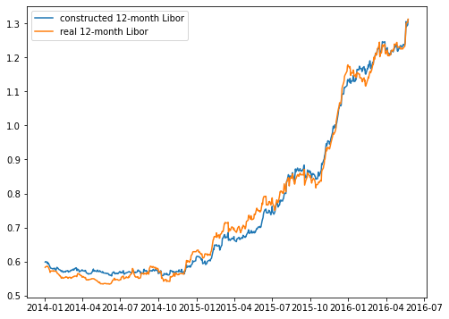
Let’s compute the fitted values $\hat y$ and plot them side to side the real $y$.

y_hat = b_0 + x.US0002M * b_1 + x.US0003M * b_2 + x.US0006M * b_3
plt.figure(figsize=(8,6))
plt.plot(sub_df.Date, y_hat)
plt.plot(sub_df.Date, y)
plt.legend(['constructed 12-month Libor', 'real 12-month Libor'])
plt.show()

png

The mean squared error surface and its gradient

For visualization purposes, we will work on the case of simple regression, that is

$y = b_0 + b_1 x + \epsilon$.

Assume that you have $n$ data points $(x_1,y_1), \ldots, (x_n, y_n)$. We define the mean squared error (MSE) as

$f(b_0,b_1) = \frac{1}{n}\sum_{i=1}^n \left(y_i - (b_0 + b_1 x_i) \right)^2$.

Observe that here the data $(x_i,y_i)$ is fixed and the MSE is a quadratic function of the variables $(b_0, b_1)$. Then, the linear regression coefficients are the pair $(b_0^*, b_1^*)$ which minimizes $f(b_0, b_1)$.

Assume that the target variable is the 12-month Libor rate, i.e. $y=L_12$, the regressor is the 1-month Libor rate, i.e. $x=L_1$, and the data consists of the observation from 2016-01-01 to 2017-12-31.

Q9. What is the value of $f(0,0)$?
Q10. What is the value of $f(-100,-100)$?
Q11. What is the value of $f(100,25)$?
Q12. What is the value of $∂f(b_0,b_1)/∂b_0$ evaluated at $(b_0, b_1)=(0,0)$?
Q13. What is the value of $∂f(b_0,b_1)/∂b_1$ evaluated at $(b_0, b_1)=(0,0)$?
Q14. What is the value of $∂f(b_0,b_1)/∂b_0$ evaluated at $(b_0, b_1)=(-100,-100)$?
Q15. What is the value of $∂f(b_0,b_1)/∂b_1$ evaluated at $(b_0, b_1)=(-100,-100)$?

First, we fix a time window and extract the data.

# we fix a time window
d1 = '2016-01-01'
d2 = '2017-12-31'

# we extract the data for the time window
sub_df = libor_rates_time_window(df, d1, d2)

In this case, the target variable is the 12-month Libor and the regressor is the 1-month Libor.

# simple regression (6-month Libor against 2-month Libor)
x = np.array(sub_df.US0001M)
y = np.array(sub_df.US0012M)

Now, write a function that given data x and y and parameters computes $f(b_0, b_1)$. Don’t forget to divide by the number of points $n$!

def mean_sq_err(b_vector, x, y):
    ''' Computes the MSE (linear regression) given data x and y. '''
    # extract b's
    b_0 = b_vector[0]
    b_1 = b_vector[1]
    
    mse = 0.

    x = np.array(x)
    y = np.array(y)
    err = y - b_0 - b_1 * x
    n = len(x)
    mse = np.sum(np.square(err)) / n
    
    return mse

# question 9
b_0 = 0.0
b_1 = 0.0
b_vec = np.array([b_0, b_1])
mse = mean_sq_err(b_vec, x, y)
print('MSE = ' + str(np.round(mse,4)))

MSE = 2.5651

# question 10
b_0 = -100.
b_1 = -100.
b_vec = np.array([b_0, b_1])
mse = mean_sq_err(b_vec, x, y)
print('MSE = ' + str(np.round(mse,2)))

MSE = 34334.38

# question 11
b_0 = 100.
b_1 = 25.
b_vec = np.array([b_0, b_1])
mse = mean_sq_err(b_vec, x, y)
print('MSE = ' + str(np.round(mse,2)))

MSE = 14118.26

We now draw the countours of $f(b_0, b_1)$. For this we need to evaluate $f(b_0, b_1)$ on a grid of values of $b_0$ and $b_1$.

# define range for b_0 and b_1
lim = 200
space = 5
b_0_range = np.arange(-lim, lim + space, space)
len1 = len(b_0_range)
b_1_range = np.arange(-lim, lim + space, space)
len2 = len(b_1_range)
# here we store the values of f
f_grid = np.zeros((len2, len1))
# we create a grid
b_0_grid, b_1_grid = np.meshgrid(b_0_range, b_1_range)
# compute error surface
for i in range(len1):
    for j in range(len2):
        b_vec = np.array([b_0_grid[j, i], b_1_grid[j, i]])
        f_grid[j, i] = mean_sq_err(b_vec, x, y)

# plot the countours of the MSE
plt.figure(figsize=(8,5)) # set the figure size
plt.contour(b_0_grid, b_1_grid, f_grid,40)
plt.xlabel('b_0')
plt.ylabel('b_1')
plt.show()

png

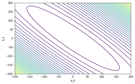
The linear coefficients $(b_0^*, b_1^*)$ lie in the center of the above surface. We will now implement a gradient descent (GD) routine to find them. Of course, in the case of linear of regression, we can compute them analytically like in the previous section. This will only be an illustration of how GD works.

Before implementing GD, write a function that computes the gradient of $f(b_0, b_1)$. Recall that the gradient in this case is a 2-dimensional vector $\nabla_f = \left( \frac{\partial f(b_0,b_1)}{\partial b_0}, \frac{\partial f(b_0,b_1)}{\partial b_1 }\right)$.

def gradient_mse(b_vector, x, y):
    ''' Computes the gradient of the MSE given data x and y. '''
    # extract b's
    b_0 = b_vector[0]
    b_1 = b_vector[1]
    
    grad = np.zeros(2)


    x = np.array(x)
    y = np.array(y)
    err = y - b_0 - b_1 * x
    n = len(x)
    partial_b_0 = -2 * np.sum(err) / n
    partial_b_1 = -2 * np.sum(err * x) / n
    
    grad[0] = partial_b_0
    grad[1] = partial_b_1
    
    return grad

# question 12
b_0 = 0.0
b_1 = 0.0
b_vec = np.array([b_0, b_1])
grad = gradient_mse(b_vec, x, y)
print('df_db0 = ' + str(np.round(grad[0],4)))

df_db0 = -3.1628

# question 13
print('df_db1 = ' + str(np.round(grad[1],4)))

df_db1 = -2.6948

# question 14
b_0 = -100.0
b_1 = -100.0
b_vec = np.array([b_0, b_1])
grad = gradient_mse(b_vec, x, y)
print('df_db0 = ' + str(np.round(grad[0],2)))

df_db0 = -363.97

# question 15
print('df_db1 = ' + str(np.round(grad[1],2)))

df_db1 = -316.8

The learning rate and gradient descent (GD)

Now, we will code a very simplified implementation of GD. Recall that GD is an iterative procedure that updates the current the parameter vector $b^k = (b_0^k, b_1^k)$ as follows:

$b^{k+1} = b^k - \gamma \nabla_f(b^k)$,

where $\gamma > 0$ is the learning rate and $\nabla_f(b_k)$ is the gradient evaluated at the current iteration.

Do 5 iterations of gradient descent with initial point $(b_0^{(0)}, b_1^{(0)})=(-150,-150)$ and learning rate $\gamma =0.3$.

Q16. What is the value of $b_0^{(5)}$?

Q17. What is the value of $b_1^{(5)}$?

Do 10 iterations of gradient descent with initial point $(b_0^{(0)}, b_1^{(0)})=(150,50)$ and learning rate $\gamma=0.1$.

Q18. What is the value of $b_0^{(10)}$?

Q19. What is the value of $b_1^{(10)}$?

Assume that you start gradient descent at $(b_0^{(0)}, b_1^{(0)})=(175,25)$ and that you have a computational budget of at most 300 iterations. Choose a suitable learning rate $\gamma >0$ and find the minimizer $b_0^{*}, b_1^{*}$ of the MSE surface $f(b_0, b_1)$ (or at least a good approximation of it).

Q20. What is the value of $b_0^*$?

Q21. What is the value of $b_1^*$?

Let’s write a function that, given $b^k$ and $\gamma > 0$, computes $b^{k+1}$.

def step_gd(b_vec_old, gamma, x, y):
    ''' Computes one GD step. '''
    
    b_vec_new = np.zeros(2)

    grad_old = gradient_mse(b_vec_old, x, y)
    b_vec_new = b_vec_old - gamma * grad_old

    return b_vec_new

The GD implementation consists on calling the above function $m$ times, starting from an initial point $b_0$. It returns a matrix with all the iterations $b_0, b_1, \ldots, b_m$. If $m$ is sufficiently large and the learning rate $\gamma$ is adequate (not too small or large), then the sequence of $b_k$’s should converge to the optimal $b^* = (b_0^*, b_1^*)$.

def gradient_descent(b_vec0, gamma, m, x, y):
    ''' Simplified gradient descent implementation. '''
    
    b_matrix = np.zeros([m + 1, 2])
    b_matrix[0] = b_vec0
    for k in range(m):
        b_matrix[k + 1] = step_gd(b_matrix[k], gamma, x, y)      
    
    return b_matrix

# question 16
b_vec0 = [-150, -150]
gamma = 0.3
m = 5
b_vec_gd = gradient_descent(b_vec0, gamma, m, x, y)
print('b_0 = ' + str(np.round(b_vec_gd[-1][0], 4)))

b_0 = 9.0045

# question 17
print('b_1 = ' + str(np.round(b_vec_gd[-1][1], 4)))

b_1 = -8.5341

# question 18
b_vec0 = [150, 50]
gamma = 0.1
m = 10
b_vec_gd = gradient_descent(b_vec0, gamma, m, x, y)
print('b_0 = ' + str(np.round(b_vec_gd[-1][0], 4)))

b_0 = 36.9246

# question 19
print('b_1 = ' + str(np.round(b_vec_gd[-1][1], 4)))

b_1 = -37.2826

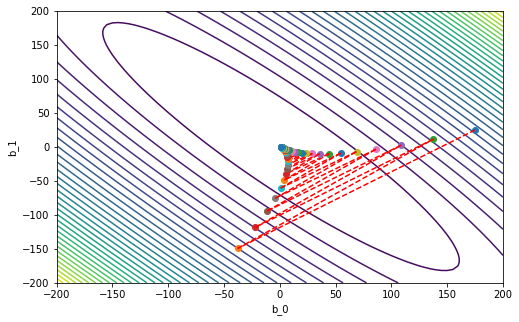
The choice of the learning rate $\gamma$ could determine the outcome of the GD. On on hand, small values of $\gamma$ will give us very slow convergence. On the other hand, large values of $\gamma$ will make the GD diverge! We test different values for $\gamma$.

# fix the initial point
b_vec0 = [175, 25]
# number of iterations
m = 300

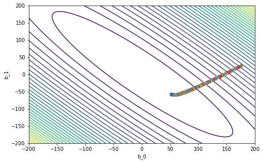
Case 1

$\gamma = 0.005$

gamma = 0.005
b_vec_gd = gradient_descent(b_vec0, gamma, m, x, y)
# this is the last point
print('b_m = ' + str(b_vec_gd[-1]))

b_m = [ 52.20228377 -57.12526282]

# plot the countours of the MSE
plt.figure(figsize=(8,5)) # set the figure size
plt.contour(b_0_grid, b_1_grid, f_grid,40)
plt.xlabel('b_0')
plt.ylabel('b_1')

# plot our GD iterations
plt.plot(b_vec_gd[0,0], b_vec_gd[0,1], 'o')
for k in range(m):
    plt.plot(b_vec_gd[k+1,0], b_vec_gd[k+1,1], 'o')
    plt.plot(b_vec_gd[k : k+2, 0], b_vec_gd[k : k+2, 1], '--r')

plt.show()

png

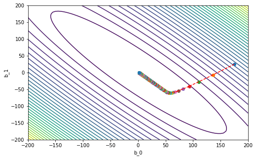
Case 2

$\gamma = 0.1$

gamma = 0.1
b_vec_gd = gradient_descent(b_vec0, gamma, m, x, y)
# this is the last point
print('b_m = ' + str(b_vec_gd[-1]))

b_m = [ 1.94081301 -0.3706432 ]

# plot the countours of the MSE
plt.figure(figsize=(8,5)) # set the figure size
plt.contour(b_0_grid, b_1_grid, f_grid,40)
plt.xlabel('b_0')
plt.ylabel('b_1')

# plot our GD iterations
plt.plot(b_vec_gd[0,0], b_vec_gd[0,1], 'o')
for k in range(m):
    plt.plot(b_vec_gd[k+1,0], b_vec_gd[k+1,1], 'o')
    plt.plot(b_vec_gd[k : k+2, 0], b_vec_gd[k : k+2, 1], '--r')

plt.show()

png

Case 3

$\gamma = 0.55$

gamma = 0.55
b_vec_gd = gradient_descent(b_vec0, gamma, m, x, y)
# this is the last point
print('b_m = ' + str(b_vec_gd[-1]))

b_m = [1.07304106 0.63223684]

# plot the countours of the MSE
plt.figure(figsize=(8,5)) # set the figure size
plt.contour(b_0_grid, b_1_grid, f_grid,40)
plt.xlabel('b_0')
plt.ylabel('b_1')

# plot our GD iterations
plt.plot(b_vec_gd[0,0], b_vec_gd[0,1], 'o')
for k in range(m):
    plt.plot(b_vec_gd[k+1,0], b_vec_gd[k+1,1], 'o')
    plt.plot(b_vec_gd[k : k+2, 0], b_vec_gd[k : k+2, 1], '--r')

plt.show()

png

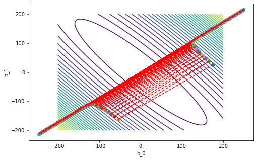
Case 4

$\gamma = 0.5905$

gamma = 0.5905
b_vec_gd = gradient_descent(b_vec0, gamma, m, x, y)
# this is the last point
print('b_m = ' + str(b_vec_gd[-1]))

b_m = [248.76153639 214.95211362]

# plot the countours of the MSE
plt.figure(figsize=(8,5)) # set the figure size
plt.contour(b_0_grid, b_1_grid, f_grid,40)
plt.xlabel('b_0')
plt.ylabel('b_1')

# plot our GD iterations
plt.plot(b_vec_gd[0,0], b_vec_gd[0,1], 'o')
for k in range(m):
    plt.plot(b_vec_gd[k+1,0], b_vec_gd[k+1,1], 'o')
    plt.plot(b_vec_gd[k : k+2, 0], b_vec_gd[k : k+2, 1], '--r')

plt.show()

png

After a visual inspection of the previous 4 cases, select a suitable value for $\gamma$.

gamma = 0.55

# question 20
b_vec0 = [175, 25]
m = 300
b_vec_gd = gradient_descent(b_vec0, gamma, m, x, y)
print('b_0_star = ' + str(np.round(b_vec_gd[-1, 0], 4)))

b_0_star = 1.073

print('b_1_star = ' + str(np.round(b_vec_gd[-1, 1], 4)))

b_1_star = 0.6322

In this tutorial, we: fit a linear model in Python; computed the $R^2$ of the regression; visually compared real vs fitted values; implemented a simple gradient descent (GD) optimization routine; appreciated the importance of the learning rate of the GD.