This tutorial is a guide for a data analysis on the Libor rates data (similar to the one done in class for swap rates).
C’est un support des travaux dirigés pour le cours de M2 “Financial Engineering and Risk Management” que j’ai enseigné aux étudiants de l’Université Paris-Sud en 2017 et 2018 (devenue désormais Paris-Saclay).
Using the data from the file “swapLiborData.csv” , answer the following questions.
Q1. What was the 2-month Libor rate on 2015-03-31?
Q2. What was the 6-month Libor rate on 2017-12-12?
Q3. What was the 12-month Libor rate on 2018-05-25?
Let’s import Python modules and read the data.
import numpy as np # for fast vector computations
import pandas as pd # for easy data analysis
import matplotlib.pyplot as plt # for plotting
from sklearn import linear_model # for linear regression
# load data using pandas
df = pd.read_csv('3.swapLiborData.csv')
We print the first rows of a dataframe.
df.head()
| Date | US0001M | US0002M | US0003M | US0006M | US0012M | USSW2 | USSW3 | USSW5 | USSW7 | USSW10 | USSW15 | USSW30 | |
|---|---|---|---|---|---|---|---|---|---|---|---|---|---|
| 0 | 41641 | 0.1683 | 0.21250 | 0.24285 | 0.3464 | 0.5826 | 0.4903 | 0.8705 | 1.7740 | 2.4540 | 3.0610 | 3.5613 | 3.8950 |
| 1 | 41642 | 0.1647 | 0.20995 | 0.23985 | 0.3452 | 0.5846 | 0.5113 | 0.9000 | 1.7920 | 2.4648 | 3.0665 | 3.5635 | 3.8953 |
| 2 | 41645 | 0.1625 | 0.20825 | 0.23935 | 0.3445 | 0.5854 | 0.5000 | 0.8760 | 1.7468 | 2.4203 | 3.0260 | 3.5315 | 3.8738 |
| 3 | 41646 | 0.1615 | 0.20820 | 0.24210 | 0.3447 | 0.5866 | 0.4985 | 0.8735 | 1.7375 | 2.4065 | 3.0098 | 3.5145 | 3.8580 |
| 4 | 41647 | 0.1610 | 0.20750 | 0.24040 | 0.3452 | 0.5856 | 0.5350 | 0.9520 | 1.8280 | 2.4835 | 3.0650 | 3.5500 | 3.8703 |
The ‘Date’ variable in the original file is in numeric format. We transform it into a more readable year-month-day format.
df['Date'] = pd.to_datetime('1899-12-30') + pd.to_timedelta(df['Date'],'D')
df.head()
| Date | US0001M | US0002M | US0003M | US0006M | US0012M | USSW2 | USSW3 | USSW5 | USSW7 | USSW10 | USSW15 | USSW30 | |
|---|---|---|---|---|---|---|---|---|---|---|---|---|---|
| 0 | 2014-01-02 | 0.1683 | 0.21250 | 0.24285 | 0.3464 | 0.5826 | 0.4903 | 0.8705 | 1.7740 | 2.4540 | 3.0610 | 3.5613 | 3.8950 |
| 1 | 2014-01-03 | 0.1647 | 0.20995 | 0.23985 | 0.3452 | 0.5846 | 0.5113 | 0.9000 | 1.7920 | 2.4648 | 3.0665 | 3.5635 | 3.8953 |
| 2 | 2014-01-06 | 0.1625 | 0.20825 | 0.23935 | 0.3445 | 0.5854 | 0.5000 | 0.8760 | 1.7468 | 2.4203 | 3.0260 | 3.5315 | 3.8738 |
| 3 | 2014-01-07 | 0.1615 | 0.20820 | 0.24210 | 0.3447 | 0.5866 | 0.4985 | 0.8735 | 1.7375 | 2.4065 | 3.0098 | 3.5145 | 3.8580 |
| 4 | 2014-01-08 | 0.1610 | 0.20750 | 0.24040 | 0.3452 | 0.5856 | 0.5350 | 0.9520 | 1.8280 | 2.4835 | 3.0650 | 3.5500 | 3.8703 |
Much better!
Libor rates and plotting curves
Let’s write a function that given the dataframe and a date such as ‘2014-01-08’ returns a vector of length 5 with the libor rates for that date (1, 2, 3, 6, and 12 months). You can assume that the date given can always be found in the data.
def libor_rates_date(df, date):
    ''' Retrieve the Libor rates (all terms) for a given date. '''

    libor_rates = np.zeros(5)


    temp = df[df['Date'] == date].iloc[0,1:6]
    libor_rates = np.array(temp, dtype='float')

    return libor_rates
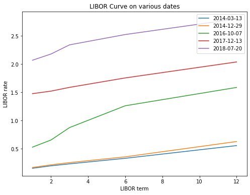
Let’s plot the libor rates for these 5 dates:
dates = ['2014-03-13', '2014-12-29', '2016-10-07', '2017-12-13', '2018-07-20']
plt.figure(figsize=(8,6)) # you can change the size to fit better your screen

for d in dates:
    plt.plot([1, 2, 3, 6 ,12], libor_rates_date(df, d)) # plot rates

# labels, title and legends
plt.xlabel('LIBOR term')
plt.ylabel('LIBOR rate')
plt.title('LIBOR Curve on various dates')
plt.legend(dates)

plt.show()
Now, let’s write a function that returns the Libor rate for a specific date and term (in months). The term can be any of the following integers: 1, 2, 3, 6, 12. Hint: you can use the previous function ‘libor_rates_date’ as part of your code.
def libor_rate_date_term(df, date, term):
    ''' Retrieve the Libor rate for a given date and term. '''

    libor = 0.


    libors = libor_rates_date(df, date)
    if term == 1:
        libor = libors[0]
    elif term == 2:
        libor = libors[1]
    elif term == 3:
        libor = libors[2]
    elif term == 6:
        libor = libors[3]
    elif term == 12:
        libor = libors[4]

    return libor
Use the previous function to find the following swap rates. Input them manually on the quiz page (rounded to 4 decimals). Of course! You could manually inspect the table to find the correct rate, but that would not be any fun!
# question 1
date = '2015-03-31'
term = 2
libor_rate = libor_rate_date_term(df, date, term)
print(np.round(libor_rate,4))
0.2218
# question 2
date = '2017-12-12'
term = 6
libor_rate = libor_rate_date_term(df, date, term)
print(np.round(libor_rate,4))
1.7477
# question 3
date = '2018-05-25'
term = 12
libor_rate = libor_rate_date_term(df, date, term)
print(np.round(libor_rate,4))
2.7314
Computing Libor rates correlations
Using the historical swap and Libor rate data from “swapLiborData.csv”, answer the following questions:
Q4. What was the correlation between the 1-month Libor rate and 3-month Libor rate from 2014-01-01 to 2015-12-31?
Q5. What was the correlation between the 1-month Libor rate and 12-month Libor rate from 2016-01-01 to 2017-12-31?
Q6. What was the correlation between the 2-month Libor rate and 6-month Libor rate from 2018-01-01 to 2018-10-11?
We are now interested in computing correlations between different Libor rates over certain time windows. For this analysis, write a function that given two dates d1 <= d2, returns a dataframe with all the libor rates in that time interval.
def libor_rates_time_window(df, d1, d2):
    ''' Retrieve the Libor rates (all terms) for the date window d1 to d2. '''

    sub_df = pd.DataFrame()


    sub_df = df[df['Date'] >= d1]
    sub_df = sub_df[sub_df['Date'] <= d2]
    sub_df = sub_df.iloc[:,:6]


    return sub_df
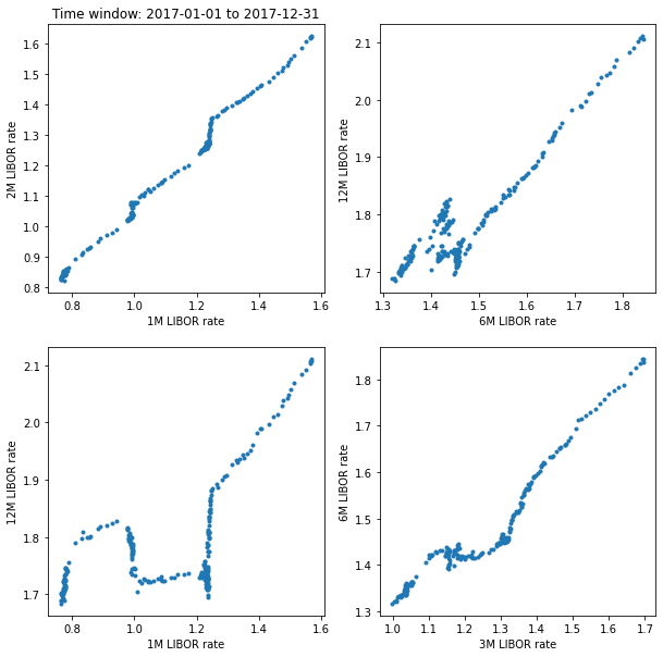
Let’s use the previous function to do some scatter plots.
def scatter_plot_window(df, d1, d2):
    ''' Plots scatter plots for a time window. '''

    df_sub = libor_rates_time_window(df, d1, d2)

    plt.figure(figsize=(10,10))

    plt.subplot(2,2,1)
    plt.title('Time window: ' + d1 + ' to ' + d2)
    plt.plot(df_sub.US0001M, df_sub.US0002M, '.')
    plt.xlabel('1M LIBOR rate')
    plt.ylabel('2M LIBOR rate')

    plt.subplot(2,2,2)
    plt.plot(df_sub.US0006M, df_sub.US0012M, '.')
    plt.xlabel('6M LIBOR rate')
    plt.ylabel('12M LIBOR rate')

    plt.subplot(2,2,3)
    plt.plot(df_sub.US0001M, df_sub.US0012M, '.')
    plt.xlabel('1M LIBOR rate')
    plt.ylabel('12M LIBOR rate')

    plt.subplot(2,2,4)
    plt.plot(df_sub.US0003M, df_sub.US0006M, '.')
    plt.xlabel('3M LIBOR rate')
    plt.ylabel('6M LIBOR rate')

    plt.show()
For example, let’s see the scatter plots for 2017.
scatter_plot_window(df, '2017-01-01', '2017-12-31')
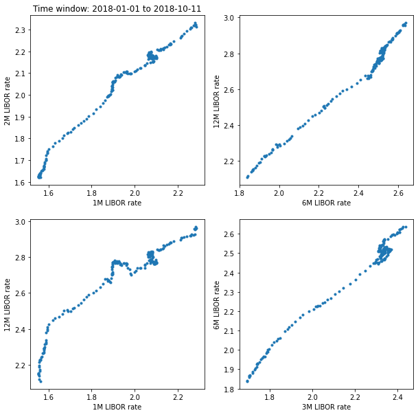
And now for 2018.
scatter_plot_window(df, '2018-01-01', '2018-10-11')
Finally, write a function that given a time window [d1, d2] and two Libor terms (in months) t1 and t2 returns the correlation of the corresponding Libor rates during that window. t1 and t2 can only take the values: 1,2,3,6,12. Hint: use the previous function ‘libor_rates_time_window’ and the Pandas function pd.df.corr() to compute the correlation.
def corr_window(df, d1, d2, term1, term2):

    corr = 0.0


    if term1 == term2:
        corr = 1.
        return corr

    def col_name(term):
        if term == 12:
            return 'US0012M'
        else:
            return 'US000' + str(term) + 'M'

    col_name_1 = col_name(term1)
    col_name_2 = col_name(term2)
    df_sub = libor_rates_time_window(df[['Date', col_name_1, col_name_2]], d1, d2)
    df_corr = df_sub.corr()
    corr = df_corr.iloc[0,1]


    return corr
Use the previous function to compute the following correlations. Input them manually on the quiz page (rounded to 3 decimals).
# question 4
date1 = '2014-01-01'
date2 = '2015-12-31'
libor_term1 = 1
libor_term2 = 3
corr = corr_window(df, date1, date2, libor_term1, libor_term2)
print(np.round(corr, 3))
0.972
# question 5
date1 = '2016-01-01'
date2 = '2017-12-31'
libor_term1 = 1
libor_term2 = 12
corr = corr_window(df, date1, date2, libor_term1, libor_term2)
print(np.round(corr, 3))
0.864
# question 6
date1 = '2018-01-01'
date2 = '2018-10-11'
libor_term1 = 2
libor_term2 = 6
corr = corr_window(df, date1, date2, libor_term1, libor_term2)
print(np.round(corr, 3))
0.967