This tutorial gives hands-on experience on descriptive analysis (visualization, implied volatility) for option pricing, and model calibration on virtual option data (finding optimal initial start point for optimization routine, calibrating stochastic models on a dataset). The term “virtual option” means the option that do not exist in real market, but instead simulated from stochastic models.
C’est un support des travaux dirigés pour le cours de M2 “Financial Engineering and Risk Management” que j’ai enseigné aux étudiants de l’Université Paris-Sud en 2017 et 2018 (devenue désormais Paris-Saclay).
Calculating the implied volatility
Given Apple’s call option bid and ask data, calculate the implied volatility for the following call option and put option. Note: The implied volatility is the volatility that makes the option price from BS model equal to its actual market price.
\(K = 190\)
\(T-t = 151/365\)
\(q = 0.005\)
\(r = 0.0245\)
\(S_0 = 190.3\)
\(C = 10.875\)
\(P = 9.625\)
We import necessary modules:
import warnings
warnings.filterwarnings("ignore")

import numpy as np
import pandas as pd
import matplotlib.pyplot as plt
from matplotlib import cm
%matplotlib inline
# for interactive figures
#%matplotlib notebook
from mpl_toolkits.mplot3d import Axes3D
from scipy import interpolate
from scipy.stats import norm
from scipy import optimize
import cmath
import math
Let’s load data from Excel:
# file name
excel_file = 'data_apple.xlsx'
# read data into a data frame
df = pd.read_excel(excel_file)
# create the 'Mid' variable
df['Mid'] = df[['Bid','Ask']].mean(axis=1)
# see some of the data
df.head()
| Option_type | Maturity_days | Strike | Ticker | Bid | Ask | Last | IVM | Volm | Mid | |
|---|---|---|---|---|---|---|---|---|---|---|
| 0 | Call | 25 | 170.0 | AAPL 8/17/18 C170 | 21.150000 | 21.400000 | 20.65 | 30.762677 | 7 | 21.275000 |
| 1 | Call | 25 | 172.5 | AAPL 8/17/18 C172.5 | 18.649994 | 19.049988 | 0.00 | 29.173643 | 0 | 18.849991 |
| 2 | Call | 25 | 175.0 | AAPL 8/17/18 C175 | 16.449997 | 16.649994 | 16.50 | 28.306871 | 19 | 16.549995 |
| 3 | Call | 25 | 177.5 | AAPL 8/17/18 C177.5 | 14.100000 | 14.400000 | 0.00 | 26.967507 | 0 | 14.250000 |
| 4 | Call | 25 | 180.0 | AAPL 8/17/18 C180 | 12.050000 | 12.150000 | 12.10 | 26.321682 | 1129 | 12.100000 |
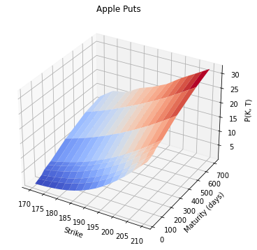
Plotting put options surface
Let’s plot put options surface for the given AAPL data. We use linear interpolation for missing strikes.
# define strikes and maturities
#all_strikes = np.sort(df_calls.Strike.unique())
all_strikes = np.arange(170., 210. + 2.5, 2.5)
all_maturities = np.sort(df.Maturity_days.unique())
print(all_strikes)
print(all_maturities)
[170.  172.5 175.  177.5 180.  182.5 185.  187.5 190.  192.5 195.  197.5
 200.  202.5 205.  207.5 210. ]
[ 25  60  88 116 151 179 333 543 697]
df_puts = df[df['Option_type'] == 'Put'][['Maturity_days', 'Strike', 'Mid']]
df_puts.head()
| Maturity_days | Strike | Mid | |
|---|---|---|---|
| 17 | 25 | 170.0 | 0.435 |
| 18 | 25 | 172.5 | 0.570 |
| 19 | 25 | 175.0 | 0.765 |
| 20 | 25 | 177.5 | 1.035 |
| 21 | 25 | 180.0 | 1.415 |
# define a grid for the surface
X, Y = np.meshgrid(all_strikes, all_maturities)
Z_p = np.empty([len(all_maturities), len(all_strikes)])
# Use linear interpolation to fill missing strikes
for i in range(len(all_maturities)):
    maturity_data = df_puts[df_puts['Maturity_days'] == all_maturities[i]]

    # Interpolate for the mid prices
    interp_func = interpolate.interp1d(maturity_data['Strike'], maturity_data['Mid'], kind='linear', fill_value="extrapolate")

    # Fill the grid with interpolated values
    Z_p[i, :] = interp_func(all_strikes)
# plot the surface
fig = plt.figure(figsize=(8,6))
ax = fig.add_subplot(111, projection='3d')
ax.plot_surface(X, Y, Z_p, cmap=cm.coolwarm)
ax.set_ylabel('Maturity (days)')
ax.set_xlabel('Strike')
ax.set_zlabel('P(K, T)')
ax.set_title('Apple Puts')
plt.savefig('fig3.png')
plt.show()
Calculate implied volatility
Calculate the implied volatility of the following call option and put option. The implied volatility is the volatility that makes the option price from BS model equal to its actual market price.
\(K\) = 190
\(T-t\) = 151/365
\(q\) = 0.005
\(r\) = 0.0245
\(S_0\) = 190.3
\(C\) = 10.875
\(P\) = 9.625
# select strike and maturity
K = 190.
T_days = 151
T_years = 1.* T_days / 365

# dividend rate
q = 0.005

# risk free rate
r = 0.0245

# spot price
S_0 = 190.3

# price
P_call = 10.875
P_put = 9.625
# utilize the following black scholes calculator to get the price from BS model
def BS_d1(S, K, r, q, sigma, tau):
    ''' Computes d1 for the Black Scholes formula '''
    d1 = 1.0*(np.log(1.0 * S/K) + (r - q + sigma**2/2) * tau) / (sigma * np.sqrt(tau))
    return d1

def BS_d2(S, K, r, q, sigma, tau):
    ''' Computes d2 for the Black Scholes formula '''
    d2 = 1.0*(np.log(1.0 * S/K) + (r - q - sigma**2/2) * tau) / (sigma * np.sqrt(tau))
    return d2

def BS_price(type_option, S, K, r, q, sigma, T, t=0):
    ''' Computes the Black Scholes price for a 'call' or 'put' option '''
    tau = T - t
    d1 = BS_d1(S, K, r, q, sigma, tau)
    d2 = BS_d2(S, K, r, q, sigma, tau)
    if type_option == 'call':
        price = S * np.exp(-q * tau) * norm.cdf(d1) - K * np.exp(-r * tau) * norm.cdf(d2)
    elif type_option == 'put':
        price = K * np.exp(-r * tau) * norm.cdf(-d2) - S * np.exp(-q * tau) * norm.cdf(-d1)
    return price

### part need to be finished ###
# auxiliary function for computing implied vol
def aux_imp_vol(sigma, P, type_option, S, K, r, q, T, t=0):

    # Calculate the Black-Scholes price
    bs_price = BS_price(type_option, S, K, r, q, sigma, T, t)
    # Return the difference between the market price and the BS price
    return bs_price - P
# compute implied vol
imp_vol_call = optimize.brentq(aux_imp_vol, 0.01, 0.4, args=(P_call, 'call', S_0, K, r, q, T_years))
imp_vol_put = optimize.brentq(aux_imp_vol, 0.01, 0.4, args=(P_put, 'put', S_0, K, r, q, T_years))
imp_vol_call, imp_vol_put
(0.20505479848219343, 0.2169237544182971)
Answer: the implied volatilities of the options are:
call: 0.2051
put: 0.2169
Heston model: searching optimal initial point
Given two sets of initial parameters of Heston model, \(P_1 = (1.0, 0.02, 0.05, -0.4, 0.08), P_2 = (3.0, 0.06, 0.10, -0.6, 0.04)\), find the optimal initial parameters set lying on the hyperparameter line between the given two parameters sets.
# import module needed for option pricing
import readPlotOptionSurface
import modulesForCalibration as mfc

# Parameters
alpha = 1.5
eta = 0.2

n = 12

# Model
model = 'Heston'


# risk free rate
r = 0.0245
# dividend rate
q = 0.005
# spot price
S0 = 190.3
params1 = (1.0, 0.02, 0.05, -0.4, 0.08)
params2 = (3.0, 0.06, 0.10, -0.6, 0.04)
iArray = []
rmseArray = []
rmseMin = 1e10

maturities, strikes, callPrices = readPlotOptionSurface.readNPlot()

marketPrices = callPrices
maturities_years = maturities/365.0
from scipy.optimize import minimize_scalar
#  Note: You could use the eValue function in modulesForCalibration (mfc) to calculate the mean square error.
#  For more detail about this function, please refer to modulesForCalibration.py

# Initialize optimal parameters and minimum RMSE
optimParams = params1
rmseMin = 10**6

# Initialize the search for optimal parameters between params1 and params2
kappa_range = np.linspace(params1[0], params2[0], num= int((params2[0]-params1[0])/0.01) + 1)

# Iterate through the parameter grid

def f(kappa):
    theta = params1[1] + (kappa - params1[0])/(params2[0] - params1[0])*(params2[1] - params1[1])
    sigma = params1[2] + (kappa - params1[0])/(params2[0] - params1[0])*(params2[2] - params1[2])
    rho   = params1[3] + (kappa - params1[0])/(params2[0] - params1[0])*(params2[3] - params1[3])
    v0    = params1[4] + (kappa - params1[0])/(params2[0] - params1[0])*(params2[4] - params1[4])
    print("kappa", kappa)
    params = (kappa, theta, sigma, rho, v0)
    return mfc.eValue(params, marketPrices, maturities_years, strikes, r, q, S0, alpha, eta, n, model)


result = minimize_scalar(f, bounds =(params1[0], params2[0]), method="bounded")
kappa 1.7639320225002102
kappa 2.23606797749979
kappa 2.5278640450004204
kappa 2.2914719396292194
kappa 2.306021558871544
kappa 2.306683816848725
kappa 2.3065629682560886
kappa 2.3065596007108975
kappa 2.30656633580128
result
     fun: 0.8658456401462155
 message: 'Solution found.'
    nfev: 9
  status: 0
 success: True
       x: 2.3065629682560886
The min-search algorithm converged after 9 iterations at \(K=2.30\). We can now calculate the other parameters.
kappa = result["x"]
theta = params1[1] + (kappa - params1[0])/(params2[0] - params1[0])*(params2[1] - params1[1])
sigma = params1[2] + (kappa - params1[0])/(params2[0] - params1[0])*(params2[2] - params1[2])
rho   = params1[3] + (kappa - params1[0])/(params2[0] - params1[0])*(params2[3] - params1[3])
v0    = params1[4] + (kappa - params1[0])/(params2[0] - params1[0])*(params2[4] - params1[4])

theta, sigma, rho, v0
(0.046131259365121774,
 0.08266407420640222,
 -0.5306562968256089,
 0.05386874063487823)
Answer: the optimal initial parameters are:
\(K = 2.31\)
\(\theta = 0.046\)
\(\sigma = 0.083\)
\(\rho = -0.53\)
Heston Model Calibration
Calibrate the Heston model for the given dataset ‘Virtual Option Data.csv’ by brute force. The searching range of parameters should be the followings:
\(2.5 \leq \kappa \leq 3.0\) with step 2.5
\(0.06 \leq \theta \leq 0.065\) with step 0.0025
\(0.1 \leq \sigma \leq 0.3\) with step 0.05
\(-0.675 \leq \rho \leq -0.625\) with step 0.025
\(0.04 \leq v_0 \leq 0.06\) with step 0.01
What is the calibrated value of \(κ\)?
What is the calibrated value of \(θ\)?
What is the calibrated value of \(σ\)?
What is the calibrated value of \(ρ\)?
# use the following fixed Parameters to calibrate the model
S0 = 100
K = 80
k = np.log(K)
r = 0.05
q = 0.015

# Parameters setting in fourier transform
alpha = 1.5
eta = 0.2

n = 12
N = 2**n
# step-size in log strike space
lda = (2*np.pi/N)/eta

#Choice of beta
beta = np.log(S0)-N*lda/2

# Model
model = 'Heston'
# calculate characteristic function of different models
def generic_CF(u, params, T, model):

    if (model == 'GBM'):

        sig = params[0];
        mu = np.log(S0) + (r-q-sig**2/2)*T;
        a = sig*np.sqrt(T);
        phi = np.exp(1j*mu*u-(a*u)**2/2);

    elif(model == 'Heston'):

        kappa  = params[0];
        theta  = params[1];
        sigma  = params[2];
        rho    = params[3];
        v0     = params[4];

        tmp = (kappa-1j*rho*sigma*u);
        g = np.sqrt((sigma**2)*(u**2+1j*u)+tmp**2);

        pow1 = 2*kappa*theta/(sigma**2);

        numer1 = (kappa*theta*T*tmp)/(sigma**2) + 1j*u*T*r + 1j*u*math.log(S0);
        log_denum1 = pow1 * np.log(np.cosh(g*T/2)+(tmp/g)*np.sinh(g*T/2));
        tmp2 = ((u*u+1j*u)*v0)/(g/np.tanh(g*T/2)+tmp);
        log_phi = numer1 - log_denum1 - tmp2;
        phi = np.exp(log_phi);

    elif (model == 'VG'):

        sigma  = params[0];
        nu     = params[1];
        theta  = params[2];

        if (nu == 0):
            mu = math.log(S0) + (r-q - theta -0.5*sigma**2)*T;
            phi  = math.exp(1j*u*mu) * math.exp((1j*theta*u-0.5*sigma**2*u**2)*T);
        else:
            mu  = math.log(S0) + (r-q + math.log(1-theta*nu-0.5*sigma**2*nu)/nu)*T;
            phi = cmath.exp(1j*u*mu)*((1-1j*nu*theta*u+0.5*nu*sigma**2*u**2)**(-T/nu));

    return phi

# calculate option price by inverse fourier transform
def genericFFT(params, T):

    # forming vector x and strikes km for m=1,...,N
    km = []
    xX = []

    # discount factor
    df = math.exp(-r*T)

    for j in range(N):

        nuJ=j*eta
        km.append(beta+j*lda)

        psi_nuJ = df*generic_CF(nuJ-(alpha+1)*1j, params, T, model)/((alpha + 1j*nuJ)*(alpha+1+1j*nuJ))
        if j == 0:
            wJ = (eta/2)
        else:
            wJ = eta

        xX.append(cmath.exp(-1j*beta*nuJ)*psi_nuJ*wJ)

    yY = np.fft.fft(xX)

    cT_km = []
    for i in range(N):
        multiplier = math.exp(-alpha*km[i])/math.pi
        cT_km.append(multiplier*np.real(yY[i]))

    return km, cT_km

# myRange(a, b) return a generator [a, a+1, ..., b], which is different from built-in generator Range that returns [a, a+1,..., b-1].
# You may use it to perform brute force
def myRange(start, finish, increment):
    while (start <= finish):
        yield start
        start += increment
# load virtual option data
data = pd.read_csv("Virtual Option Data.csv", index_col=0)
# generate strike and maturity array
strikes = np.array(data.index, dtype=float)
maturities = np.array(data.columns, dtype=float)
marketPrices = data.values
modelPrices = np.zeros_like(marketPrices)

maeMin = 1.0e6
### part need to be finished ###

kappa_range = list(myRange(2.5, 3.0, 0.25))
theta_range = list(myRange(0.06, 0.065, 0.0025))
sigma_range = list(myRange(0.1, 0.3, 0.05))
rho_range = list(myRange(-0.675, -0.625, 0.025))
v0_range = list(myRange(0.04, 0.06, 0.01))

for kappa in kappa_range:
    print("kappa", kappa)
    for theta in theta_range:
        print("theta", theta)
        for sigma in sigma_range:
            print("sigma", sigma)
            for rho in rho_range:
                print("rho", rho)
                for v0 in v0_range:
                    print("v0", v0)
                    params = (kappa, theta, sigma, rho, v0)
                    rmse =  mfc.eValue(params, marketPrices, maturities_years, strikes, r, q, S0, alpha, eta, n, model)
                    iArray.append(params)
                    rmseArray.append(rmse)
                    print(rmse)
                    if rmse < rmseMin:
                        rmseMin = rmse
                        optimParams = params
print(rmseMin)
print(optimParams)
Answer: the calibrated values are:
\(κ = 2.75\)
\(θ = 0.06\)
\(σ = 0.25\)
\(ρ = -0.65\)