Fitzhugh-Nagumo model: an excitable system
The Fitzhugh-Nagumo model of an excitable system is a two-dimensional simplification of the Hodgkin-Huxley model of spike generation in squid giant axons.
\begin{equation} \begin{cases} \frac{dv}{dt} = v - v^3 - w + I_\text{ext}\\ \tau \frac{dw}{dt} = v - a - bw \end{cases} \end{equation}
Here $I_\text{ext}$ is a stimulus current.
We want to model the spike that is generated by a squid gian axon.
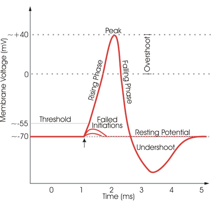
The action of an excitable neuron has the following characteristics that we knw from experiments:
- The neuron cell is initially at a resting potential value.
- If we experimentally displace the potential a little bit, it return to the resting value.
- If the perturbation is higher than a threshold value, the potential will shoot up to a very high value. In other words the spike will occur. After the spike the membrane potential will return to its resting value.
 (image from animalresearch.info)
We model the fact that the neuron as a resting potential (equilibrium for the state variable $v$). Since it is a stable equilibrium, small perturbation always leads to trajectory that converge on it. Since big perturbation start the spiking, this equilibrium cannot be unique. This is the self-excitation via a positive feedback.
Since the long term behavior of the system is to go back to the resting potential. We need a second dimension and a recovery variable that has a slower dyamics (time scale parameter $\tau$) and bring back the system toward the resting potential ($-w$ term). The recovery variable decay ($-bw$ term).
Moreover, electrophysiology show that imposing a moderate current to the membrane result in a periodic spiking. If the external current is too high, the spikes are blocked (Excitation block). Periodic spiking requires a third-degree polynomial form for the membrane potential.
Phase Diagram
from functools import partial
import numpy as np
import scipy.integrate
import scipy
import matplotlib.pyplot as plt
import matplotlib.patches as mpatches #used to write custom legends
%matplotlib inline
# Implement the flow of the Fitzhugh-Nagumo model.
# And simulate some trajectories.
# Try to use small perturbation of the resting potential as inital conditions.

scenarios = [
     {"a":-.3, "b":1.4, "tau":20, "I":0},
     {"a":-.3, "b":1.4, "tau":20, "I":0.23},
     {"a":-.3, "b":1.4, "tau":20, "I":0.5}
]
time_span = np.linspace(0, 200, num=1500)
def fitzhugh_nagumo(x, t, a, b, tau, I):
    """Time derivative of the Fitzhugh-Nagumo neural model.
    Args:
       x (array size 2): [Membrane potential, Recovery variable]
       a, b (float): Parameters.
       tau (float): Time scale.
       t (float): Time (Not used: autonomous system)
       I (float): Constant stimulus current.
    Return: dx/dt (array size 2)
    """
    pass
def fitzhugh_nagumo(x, t, a, b, tau, I):
    """Time derivative of the Fitzhugh-Nagumo neural model.
    Args:
       x (array size 2): [Membrane potential, Recovery variable]
       a, b (float): Parameters.
       tau (float): Time scale.
       t (float): Time (Not used: autonomous system)
       I (float): Constant stimulus current.
    Return: dx/dt (array size 2)
    """
    return np.array([x[0] - x[0]**3 - x[1] + I,
                     (x[0] - a - b * x[1])/tau])
def get_displacement(param, dmax=0.5,time_span=np.linspace(0,200, 1000), number=20):
    # We start from the resting point...
    ic = scipy.integrate.odeint(partial(fitzhugh_nagumo, **param),
                                                      y0=[0,0],
                                                      t= np.linspace(0,999, 1000))[-1]
    # and do some displacement of the potential.
    traj = []
    for displacement in np.linspace(0,dmax, number):
        traj.append(scipy.integrate.odeint(partial(fitzhugh_nagumo, **param),
                                                      y0=ic+np.array([displacement,0]),
                                                      t=time_span))
    return traj
# Do the numerical integration.
trajectories = {} # We store the trajectories in a dictionnary, it is easier to recover them.
for i,param in enumerate(scenarios):
    trajectories[i] = get_displacement(param, number=3, time_span=time_span, dmax=0.5)
# Draw the trajectories.
fig, ax = plt.subplots(1, len(scenarios), figsize=(5*len(scenarios),5))
for i,param in enumerate(scenarios):
        ax[i].set(xlabel='Time', ylabel='v, w',
                     title='{}'.format(param))
        for j in range(len(trajectories[i])):
            v = ax[i].plot(time_span,trajectories[i][j][:,0], color='C0')
            w = ax[i].plot(time_span,trajectories[i][j][:,1], color='C1', alpha=.5)
        ax[i].legend([v[0],w[0]],['v','w'])
plt.tight_layout()

Isoclines
Isoclines zero (or null-clines) are the manifolds on which one component of the flow is null. Find the equation of the null-clines for $v$ and $w$.
To find the null-isoclines, you have to solve:
\begin{equation} \frac{dv}{dt} = 0 \Leftrightarrow w = v - v^3 + I \end{equation}
For the first one and:
\begin{equation} \frac{dw}{dt} = 0 \Leftrightarrow w = \frac{1}{b}(v-a) \end{equation}
For the second one.
# Plot the isoclines in the phase space.
def plot_isocline(ax, a, b, tau, I, color='k', style='--', opacity=.5, vmin=-1,vmax=1):
    """Plot the null iscolines of the Fitzhugh nagumo system"""
    v = np.linspace(vmin,vmax,100)
    ax.plot(v, v - v**3 + I, style, color=color, alpha=opacity)
    ax.plot(v, (v - a)/b, style, color=color, alpha=opacity)
fig, ax = plt.subplots(1, 3, figsize=(18, 6))
for i, sc in enumerate(scenarios):
    plot_isocline(ax[i], **sc)
    ax[i].set(xlabel='v', ylabel='w',
              title='{}'.format(sc))

Flow
Let us plot the flow, which is the vector field defined by:
$F: \mathbb R^2 \mapsto \mathbb R^2$
$\vec F(v,w) = \begin{bmatrix}\frac{dv}{dt}(v,w)\\ \frac{dw}{dt}(v,w)\end{bmatrix}$
# Plot the flow using matplotlib.pyplot.streamplot.
# On the domain w \in [-1,1] and v in [-(1+a)/b, (1-a)/b]
def plot_vector_field(ax, param, xrange, yrange, steps=50):
    # Compute the vector field
    x = np.linspace(xrange[0], xrange[1], steps)
    y = np.linspace(yrange[0], yrange[1], steps)
    X,Y = np.meshgrid(x,y)

    dx,dy = fitzhugh_nagumo([X,Y],0,**param)

    # streamplot is an alternative to quiver
    # that looks nicer when your vector filed is
    # continuous.
    ax.streamplot(X,Y,dx, dy, color=(0,0,0,.1))

    ax.set(xlim=(xrange[0], xrange[1]), ylim=(yrange[0], yrange[1]))
fig, ax = plt.subplots(1, 3, figsize=(20, 6))
for i, sc in enumerate(scenarios):
    xrange = (-1, 1)
    yrange = [(1/sc['b'])*(x-sc['a']) for x in xrange]
    plot_vector_field(ax[i], sc, xrange, yrange)
    ax[i].set(xlabel='v', ylabel='w',
          title='{}'.format(sc))

Equilibrium points
The equilibria are found at the crossing between the null-isocline for $v$ and the one for $w$.
Find the polynomial equation verified by the equilibria of the model.
\begin{equation} f(v_*) = 0 = v_*^3 + v_* \left (\frac{1}{b}-1 \right ) - \frac{a}{b} \end{equation}
\begin{equation} w_* = v_* - v_*^3 + I \end{equation}
# We know that polynomial equations have at most has many roots as their degree.
# Which allow us to find all the equilibria.

# Numerically solve this equation using the function numpy.roots. Keep only the real roots.
def find_roots(a,b,I, tau):
    # The coeficients of the polynomial equation are:
    # 1           * v**3
    # 0           * v**2
    # - (1/b - 1) * v**1
    # - (a/b + I) * v**0
    coef = [1, 0, 1/b - 1, - a/b - I]

    # We are only interested in real roots.
    # np.isreal(x) returns True only if x is real.
    # The following line filter the list returned by np.roots
    # and only keep the real values.
    roots = [np.real(r) for r in np.roots(coef) if np.isreal(r)]

    # We store the position of the equilibrium.
    return [[r, r - r**3 + I] for r in roots]

eqnproot = {}
for i, param in enumerate(scenarios):
    eqnproot[i] = find_roots(**param)
Nature of the equilibria
The local nature and stability of the equilibrium is given by linearising the flow function. This is done using the Jacobian matrix of the flow:
\begin{equation} \begin{bmatrix} F_1(v+h,w+k)\\F_2(v+h,w+k) \end{bmatrix} = \begin{bmatrix} F_1(v,w)\\F_2(v,w) \end{bmatrix} + \begin{bmatrix} \frac{ \partial F_1(v,w)}{\partial v} & \frac{ \partial F_1(v,w)}{\partial w}\\ \frac{ \partial F_2(v,w)}{\partial v} & \frac{ \partial F_2(v,w)}{\partial w}\\ \end{bmatrix} \begin{bmatrix} h\\k \end{bmatrix} + o \left( \left| \left| \begin{bmatrix} h\\k \end{bmatrix} \right | \right | \right ) \end{equation}
\begin{equation} J \big \rvert_{v,w} = \begin{bmatrix} \frac{ \partial F_1(v,w)}{\partial v} & \frac{ \partial F_1(v,w)}{\partial w}\\ \frac{ \partial F_2(v,w)}{\partial v} & \frac{ \partial F_2(v,w)}{\partial w}\\ \end{bmatrix} = - \begin{bmatrix} 1 - 3 v^2 & -1 \\ \frac{1}{\tau} & -\frac{b}{\tau}\\ \end{bmatrix} \end{equation}
# Implement the jacobian of the system and use numpy.linalg.eig to determine the local topology of the equilibria.

# You can use the following color code:
EQUILIBRIUM_COLOR = {'Stable node':'C0',
                    'Unstable node':'C1',
                    'Saddle':'C4',
                    'Stable focus':'C3',
                    'Unstable focus':'C2',
                    'Center':'C5'}
def jacobian_fitznagumo(v, w, a, b, tau, I):
    """ Jacobian matrix of the ODE system modeling Fitzhugh-Nagumo's excitable system

    Args:
        v (float): Membrane potential
        w (float): Recovery variable
        a,b (float): Parameters
        tau (float): Recovery timescale.
    Return: np.array 2x2"""
def jacobian_fitznagumo(v, w, a, b, tau, I):
    """ Jacobian matrix of the ODE system modeling Fitzhugh-Nagumo's excitable system
    Args
    ====
        v (float): Membrane potential
        w (float): Recovery variable
        a,b (float): Parameters
        tau (float): Recovery timescale.
    Return: np.array 2x2"""
    return np.array([[- 3 * v**2 + 1 , -1],
                       [1/tau, -b/tau]])
# Symbolic computation of the Jacobian using sympy...
import sympy
sympy.init_printing()

# Define variable as symbols for sympy
v, w = sympy.symbols("v, w")
a, b, tau, I = sympy.symbols("a, b, tau, I")

# Symbolic expression of the system
dvdt = v - v**3 - w + I
dwdt = (v - a - b * w)/tau

# Symbolic expression of the matrix
sys = sympy.Matrix([dvdt, dwdt])
var = sympy.Matrix([v, w])
jac = sys.jacobian(var)

# You can convert jac to a function:
jacobian_fitznagumo_symbolic = sympy.lambdify((v, w, a, b, tau, I), jac, dummify=False)

#jacobian_fitznagumo = jacobian_fitznagumo_symbolic
jac
def stability(jacobian):
    """ Stability of the equilibrium given its associated 2x2 jacobian matrix.
    Use the eigenvalues.
    Args:
        jacobian (np.array 2x2): the jacobian matrix at the equilibrium point.
    Return:
        (string) status of equilibrium point.
    """

    eigv = np.linalg.eigvals(jacobian)


    if all(np.real(eigv)==0) and all(np.imag(eigv)!=0):
        nature = "Center"
    elif np.real(eigv)[0]*np.real(eigv)[1]<0:
        nature = "Saddle"
    else:
        stability = 'Unstable' if all(np.real(eigv)>0) else 'Stable'
        nature = stability + (' focus' if all(np.imag(eigv)!=0) else ' node')
    return nature

def stability_alt(jacobian):
    """ Stability of the equilibrium given its associated 2x2 jacobian matrix.
    Use the trace and determinant.
    Args:
        jacobian (np.array 2x2): the jacobian matrix at the equilibrium point.
    Return:
        (string) status of equilibrium point.
    """

    determinant = np.linalg.det(jacobian)
    trace = np.matrix.trace(jacobian)
    if np.isclose(trace, 0):
        nature = "Center (Hopf)"
    elif np.isclose(determinant, 0):
        nature = "Transcritical (Saddle-Node)"
    elif determinant < 0:
        nature = "Saddle"
    else:
        nature = "Stable" if trace < 0 else "Unstable"
        nature += " focus" if (trace**2 - 4 * determinant) < 0 else " node"
    return nature
eqstability = {}
for i, param in enumerate(scenarios):
    eqstability[i] = []
    for e in eqnproot[i]:
        J = jacobian_fitznagumo(e[0],e[1], **param)
        eqstability[i].append(stability(J))
eqstability
Complete phase diagram
def plot_phase_diagram(param, ax=None, title=None):
    """Plot a complete Fitzhugh-Nagumo phase Diagram in ax.
    Including isoclines, flow vector field, equilibria and their stability"""
    if ax is None:
        ax = plt.gca()
    if title is None:
        title = "Phase space, {}".format(param)

    # ( ... )
def plot_phase_diagram(param, ax=None, title=None):
    """Plot a complete Fitzhugh-Nagumo phase Diagram in ax.
    Including isoclines, flow vector field, equilibria and their stability"""
    if ax is None:
        ax = plt.gca()
    if title is None:
        title = "Phase space, {}".format(param)

    ax.set(xlabel='v', ylabel='w', title=title)

    # Isocline and flow...
    xlimit = (-1.5, 1.5)
    ylimit = (-.6, .9)
    plot_vector_field(ax, param, xlimit, ylimit)
    plot_isocline(ax, **param, vmin=xlimit[0],vmax=xlimit[1])

    # Plot the equilibria
    eqnproot = find_roots(**param)
    eqstability = [stability(jacobian_fitznagumo(e[0],e[1], **param)) for e in eqnproot]
    for e,n in zip(eqnproot,eqstability):
        ax.scatter(*e, color=EQUILIBRIUM_COLOR[n])

        # Show a small perturbation of the stable equilibria...
        time_span = np.linspace(0, 200, num=1500)
        if n[:6] == 'Stable':
            for perturb in (0.1, 0.6):
                ic = [e[0]+abs(perturb*e[0]),e[1]]
                traj = scipy.integrate.odeint(partial(fitzhugh_nagumo, **param),
                                                  y0=ic,
                                                  t=time_span)
                ax.plot(traj[:,0], traj[:,1])

    # Legend
    labels = frozenset(eqstability)
    ax.legend([mpatches.Patch(color=EQUILIBRIUM_COLOR[n]) for n in labels], labels,
           loc='lower right')
fig, ax = plt.subplots(1,3, figsize=(20, 6))
for i, param in enumerate(scenarios):
    plot_phase_diagram(param, ax[i])

Bifurcation diagram
# Plot the bifurcation diagram for v with respect to parameter I.

ispan = np.linspace(0,0.5,200)
bspan = np.linspace(0.6,2,200)
Bifucation on the external stimulus I
I_list = []
eqs_list = []
nature_legends = []
trace = []
det = []

for I in ispan:
    param = {'I': I, 'a': -0.3, 'b': 1.4, 'tau': 20}
    roots = find_roots(**param)
    for v,w in roots:
        J = jacobian_fitznagumo(v,w, **param)
        nature = stability(J)
        nature_legends.append(nature)
        I_list.append(I)
        eqs_list.append(v)
        det.append(np.linalg.det(J))
        trace.append(J[0,0]+J[1,1])
fig, ax = plt.subplots(1,1,figsize=(10,5))
labels = frozenset(nature_legends)
ax.scatter(I_list, eqs_list, c=[EQUILIBRIUM_COLOR[n] for n in nature_legends], s=5.9)
ax.legend([mpatches.Patch(color=EQUILIBRIUM_COLOR[n]) for n in labels], labels,
               loc='lower right')
ax.set(xlabel='External stimulus, $I_{ext}$',
       ylabel='Equilibrium Membrane potential, $v^*$');

There are four bifurcations of codim 1 in this diagram: two fold bifurcation (saddle-node) and two Hopf bifurcations (stable focus-unstable focus).
plt.scatter(det,trace, c=[EQUILIBRIUM_COLOR[n] for n in nature_legends])
plt.grid()
x = np.linspace(0,.2)
plt.plot(x, np.sqrt(4*x),color='k')
plt.plot(x, -np.sqrt(4*x),color='k')
plt.vlines(0, -1,1, color='k')
plt.hlines(0, -0.05,x.max(), color='k')
plt.text(-0.01, -0.5, 'Fold', rotation=90)
plt.text(0.15, 0.015, 'Hopf')

plt.gca().set(xlabel='Determinant of the Jacobian', ylabel='Trace of the Jacobian')
plt.fill_between(x,0,np.sqrt(4*x), color=EQUILIBRIUM_COLOR['Unstable focus'], alpha=0.2)
plt.fill_between(x,0,-np.sqrt(4*x), color=EQUILIBRIUM_COLOR['Stable focus'], alpha=0.2)
plt.fill_between(x,-np.sqrt(4*x),-1, color=EQUILIBRIUM_COLOR['Stable node'], alpha=0.2)
plt.fill_between(x,np.sqrt(4*x),1, color=EQUILIBRIUM_COLOR['Unstable node'], alpha=0.2)
plt.fill_between([-0.05,0],-1,1, color=EQUILIBRIUM_COLOR['Saddle'], alpha=0.2)
plt.legend([mpatches.Patch(color=EQUILIBRIUM_COLOR[n]) for n in labels], labels,
               loc='lower right')
plt.title("Equilibrium trajectory in the jacobian's Trace/Determinant space")

Codim 2 bifurcation on I and b
# (*) Plot the codim 2 bifurcation diagram for v with respect to parameters I and b
# For each pair (I,b) indicate the number of equilibria and if the system has periodic heteroclinic behavior.
def plot_displacement(param, dmax=0.5, ax1=None, ax2=None, tmax=200, number=20):
    if ax1 is None or ax2 is None:
        fig, (ax1,ax2) = plt.subplots(1,2,figsize=(10,5))
    # We start from the resting point...
    time_span = np.linspace(0,tmax, 1000)
    ic = scipy.integrate.odeint(partial(fitzhugh_nagumo, **param),
                                                      y0=[0,0],
                                                      t=time_span)[-1]

    # and do some displacement of the potential.
    plot_phase_diagram(param, ax=ax2)
    for displacement in np.linspace(0,dmax, number):
        traj = scipy.integrate.odeint(partial(fitzhugh_nagumo, **param),
                                                      y0=ic+np.array([displacement,0]),
                                                      t=time_span)
        ax1.plot(time_span, traj[:,0], color='k', alpha=0.3)
        ax1.set_xlabel('Time')
        ax1.set_ylabel('Membrane Potential (v)')
        ax2.plot(traj[:,0], traj[:,1], color='C0')
# Periodic behavior only happen when there are 3 equilibria, on saddle point and two unstable (focus or node).
roots = []
periodic = []
for x,i in enumerate(ispan):
    roots.append([])
    periodic.append([])
    for y,b in enumerate(bspan):
        param = {'I': i, 'a': -0.3, 'b': b, 'tau': 20}
        r = find_roots(**param)
        stab = [stability(jacobian_fitznagumo(v,w, **param)) for v,w in r]
        # Check if none of the equilibria is stable.
        periodic[x].append(not any([x[:6]=="Stable" for x in stab]))
        roots[x].append([u[0] for u in r])
mono = []
bi = []
per = []
for x,i in enumerate(ispan):
    for y,b in enumerate(bspan):
        if len(roots[x][y]) == 1:
            mono.append((i,b))
        else:
            if not periodic[x][y]:
                bi.append((i,b))
            else:
                per.append((i,b))
plt.scatter(*zip(*mono), color='C0', marker='.' ,label='Monostable')
plt.scatter(*zip(*bi), color='C1', marker='.', label='Non Periodic')
plt.scatter(*zip(*per), color='C2', marker='.', label='Periodic')
plt.legend()


ii = 0.25
bb = 1.2
plt.scatter(ii,bb, marker='X', color='k')

plt.xlabel('External stimulus, $I_{ext}$')
plt.ylabel('Recovery parameter, $b$');
plt.show()
plot_displacement({'I': ii, 'a': -0.3, 'b': bb, 'tau': 20}, tmax=300)


Non autonomous system
So far we have considered the behavior of the system under a constant stimulus $I_{ext}$. However, it is possible to extend this model to cases where the stimulus is more complex, by making $I_{ext}$ a functio of time.
\begin{equation} \begin{cases} \frac{dv}{dt} = v - v^3 - w + I_\text{ext}(t)\\ \tau \frac{dw}{dt} = v - a - bw \end{cases} \end{equation}
Note that now the system is non-autonomous.
# Implement a non autonomous version of the Fitzhugh Nagumo Model.
# Simulate some trajectories.

# Here are a few stimulus function that you can try.
def step_stimulus(t, value, time):
    """Step stimulus for the non autonomous Fitzhugh-Nagumo model"""
    return 0 if t<time else value

def step_stimulus_2(t, values, time):
    """Step stimulus for the non autonomous Fitzhugh-Nagumo model"""
    return 0 if t<time else values[int(t//time)] if t<len(values)*time else values[-1]

def periodic_stimulus(t, magnitude, freq):
    """Periodic stimulus for the non autonomous Fitzhugh-Nagumo model"""
    return magnitude * np.sin(freq * t)

def generate_noisy(scale, steps=300, dt=1, tmax=300):
    time = np.linspace(0, tmax, num=steps)
    noise = [0]
    for i in range(len(time)-1):
        noise.append( noise[-1] + (0-noise[-1])*dt + dt*np.random.normal(loc=0, scale=scale))
    def noisy_stimulus(t):
        """Noisy stimulus for the non autonomous Fitzhugh-Nagumo model"""
        tscaled = (t/tmax)*(len(noise)-2)
        i = int(tscaled)
        return (tscaled-i)*noise[i] + (i+1-tscaled)*noise[1+i]
    return noisy_stimulus

# Some parameter sets:
step_sc = []
time_span = np.linspace(0, 500, num=1500)

step_sc.append({"a":-.3, "b":1.4, "tau":20, 'I': partial(step_stimulus, value=0.2, time=100)})
step_sc.append({"a":-.3, "b":1.4, "tau":20, 'I': partial(step_stimulus_2, values=[0.1,0.2,0.6], time=100)})
step_sc.append({"a":-.3, "b":1.4, "tau":20, 'I': partial(periodic_stimulus, magnitude=1,freq=.1)})
step_sc.append({"a":-.3, "b":1.4, "tau":20, 'I': generate_noisy(.5, tmax=time_span[-1], steps=len(time_span))})

initial_conditions = [(-0.5,-0.1), [0, -0.16016209760708508]]
def non_autonomous_fitzhugh_nagumo(x, t, a, b, tau, I):
    """Time derivative of the Fitzhugh-Nagumo neural model.
    Args:
       x (array size 2): [Membrane potential, Recovery variable]
       a, b (float): Parameters.
       tau (float): Time scale.
       t (float): Time (Not used: autonomous system)
       I (function of t): Stimulus current.
    Return: dx/dt (array size 2)
    """
    pass
def non_autonomous_fitzhugh_nagumo(x, t, a, b, tau, I):
    """Time derivative of the Fitzhugh-Nagumo neural model.
    Args:
       x (array size 2): [Membrane potential, Recovery variable]
       a, b (float): Parameters.
       tau (float): Time scale.
       t (float): Time (Not used: autonomous system)
       I (function of t): Stimulus current.
    Return: dx/dt (array size 2)
    """
    return np.array([x[0] - x[0]**3 - x[1] + I(t),
                     (x[0] - a - b * x[1])/tau])
trajectory_nonauto = {}
for i, param in enumerate(step_sc):
    flow = partial(non_autonomous_fitzhugh_nagumo, **param)
    for j, ic in enumerate(initial_conditions):
        trajectory_nonauto[i, j] = scipy.integrate.odeint(flow,
                                                          y0=ic,
                                                          t=time_span)
# Draw the trajectories.
fig, ax = plt.subplots(len(step_sc), 2, figsize=(15,15))
for i, param in enumerate(step_sc):
    for j, ic in enumerate(initial_conditions):
        ax[i, j].set(xlabel='Time', ylabel='v, w, I')
        ax[i, j].plot(time_span,[param['I'](t) for t in time_span], label='I', color='C2', alpha=0.5)
        ax[i, j].plot(time_span,trajectory_nonauto[i, j][:,0], label='v', color='C0')
        ax[i, j].legend()
plt.tight_layout()

Stochastic Differential Equation
So far we have seen continuous-time, continuous-state determinsitic systems in the form of Ordinary Differential Equations (ODE). Their stochastic counterpart are Stochastic Differential Equations (SDE).
Consider the now familiar non-autonomous ODE:
\begin{equation} \frac{dy}{dt} = f(y,t) \end{equation}
The corresponding integral equation is:
\begin{equation} y(t) = y(0) + \int_0^t f(y(s),s) ds \end{equation}
The SDE would be:
\begin{equation} Y_t = f(Y_t,t) dt + g(Y_t,t) dB_t \end{equation}
Now $Y_t$ is a random variable. $B_t$ is the standard Brownian motion. The corresponding integral equation is:
\begin{equation} y(t) = y(0) + \int_0^t f(Y_s,s) ds + \int_0^t g(Y_s,s) dB_s \end{equation}
We will use the Euler-Maruyama integration scheme.
# Implement the Euler-Maruyama integration algorithm.
def euler_maruyama(flow, noise_flow, y0, t) :
    ''' Euler-Maruyama intergration.

    Args:
        flow (function): deterministic component of the flow (f(Yt,t))
        noise_flow (function): stochastic component of the flow (g(Yt,t))
        y0 (np.array): initial condition
        t (np.array): time points to integrate.

    Return the Euler Maruyama approximation of the SDE trajectory defined by:

    y(t) = f(Y(t),t)dt + g(Yt,t)dBt
    y(0) = y0
    '''
    pass
def euler_maruyama(flow, noise_flow, y0, t) :
    ''' Euler-Maruyama intergration.

    Args:
        flow (function): deterministic component of the flow (f(Yt,t))
        noise_flow (function): stochastic component of the flow (g(Yt,t))
        y0 (np.array): initial condition
        t (np.array): time points to integrate.

    Return the Euler Maruyama approximation of the SDE trajectory defined by:

    y(t) = f(Y(t),t)dt + g(Yt,t)dBt
    y(0) = y0
    '''
    y = np.zeros((len(t),len(y0)))
    y[0] = y0
    for n,dt in enumerate(np.diff(t),1):
        y[n] = y[n-1] + flow(y[n-1],dt) * dt + noise_flow(y[n-1],dt) * np.random.normal(0,np.sqrt(dt))
    return y
# Do the simulations.
# Remember that we define f as the partial application of fitzhugh_nagumo.
time_s = np.linspace(0, 1000, num=10000)
noise_flow = lambda y,t: 0.04
stochastic = {}
trajectory = {}
for i,param in enumerate(scenarios[:2]):
    for j, ic in enumerate(initial_conditions):
        # i is key and j is value in the trajectory dictionary
        flow = partial(fitzhugh_nagumo, **param)
        stochastic[i, j] = euler_maruyama(flow,
                                          noise_flow,
                                          y0=ic,
                                          t=time_s)
        trajectory[i,j] = scipy.integrate.odeint(flow, y0=ic, t=time_s)
# Draw the trajectories.
fig, ax = plt.subplots(2, 2, figsize=(20,10))
for i,param in enumerate(scenarios[:2]):
    for j, ic in enumerate(initial_conditions):
        ax[i, j].set(xlabel='Time', ylabel='v, w', title='Trajectory of v, w, {} with init = {}'.format(param, ic),
                    xlim=(0, time_s[-1]), ylim=(-1.5, 1.5))
        ax[i, j].plot(time_s,stochastic[i, j][:,0], label='v (SDE)')
        ax[i, j].plot(time_s,trajectory[i, j][:,0], label='v (ODE)', color='C0', ls=":")
ax[0, 0].legend()

xlimit = (-1.3, 1.3)
ylimit = (-0.5, 0.5)
fig, ax = plt.subplots(1,2, figsize=(12,5))
for i, param in enumerate(scenarios[:2]):
    ax[i].set(xlabel='v', ylabel='w', title="Phase space, {}".format(param))
    plot_vector_field(ax[i], param, xlimit, ylimit)
    plot_vector_field(ax[i], param, xlimit, ylimit)
    plot_isocline(ax[i], **param, vmin=xlimit[0], vmax=xlimit[1])
    for j, ic in enumerate(initial_conditions):
        ax[i].plot(stochastic[i, j][:,0], stochastic[i, j][:,1],lw=1)
