I was recently very confused with a linear regression. More precisely, I realized that my mental model of a linear regression was completely wrong, even though linear regressions are not exactly a new thing to me.
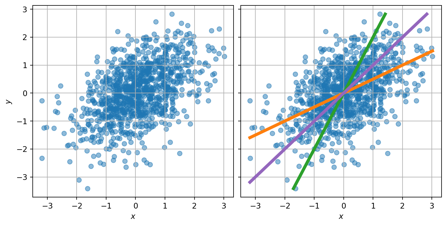
If I gave you the scatter plot below, and asked you to draw the regression line, which line would you draw? The orange, the green, or the purple one?
My intuitive answer was to draw the purple one, the one that goes through the major axis of the ellipsoid-shaped cloud. Hence my surprise when I used a statistics programming library to compute the regression, and found the orange one.
Three different regression lines
It turns out that all three answers are correct, in some way. The purple line, the one aligned with the ellipse, is defined by the eigenvectors of the covariance matrix of the data. It is also known as Deming regression. Here, I used the covariance matrix
\[\begin{pmatrix}1&\frac{1}{2}\\\frac{1}{2}&1\end{pmatrix}\]whose eigenvectors are aligned with the diagonals \(y = x\) and \(y = -x\).
But a simple linear regression is doing something different. A way I like to reason about it is to think of the residuals of the regression, i.e. \(y_i - \beta_x\,x_i\), which squares are being minimized.
What minimizes the squares of the residuals is bringing the residuals as close to zero as possible. We can see that this isn’t the case for the purple curve: for example, at \(x=2\), there are no samples above the purple curve, and plenty below. In contrast, the orange line goes through the “vertical center” of the points and results in much lower sum of squared residuals. I plotted these residuals below the same dataset with the same three lines, but where I subtract different values from \(y\). Look at how the lines and dataset seem to transform!
I think that one reason for this mismatch between what we “want” to draw, and the actual regression line, comes from the fact that it might be easier to picture ourselves a rotation of the dataset than this linear translation.
As you may have guessed, the green line is the “other” regression line: the one that regresses \(x\) on \(y\), i.e. that makes \(x_i - \beta_y\,y_i\) unbiased and independent from \(y_i\). For this one to make sense, one would need to translate points horizontally instead of vertically.
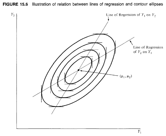
Another property of these two regression lines is that they pass through the vertical and horizontal tangents of the contour ellipses of the distribution:
The maths behind these lines
I wanted to understand the relationships between these three regression lines, so I assumed a dataset constructed as follows:
\[\begin{align*} x_i &\sim \mathrm{Normal}(0, \sigma_x)\\ y_i &\sim \mathrm{Normal}(\beta_x\,x_i, \sigma_{xy})\\ \end{align*}\]
Because of properties of the normal distribution, this creates a multivariate normal distribution with the following covariance matrix:
\[ \Sigma = \begin{pmatrix} \sigma_x^2 & \beta_x\,\sigma_x^2\\ \beta_x\,\sigma_x^2 & \beta_x^2\,\sigma_x^2+\sigma_{xy}^2\\ \end{pmatrix} \]
Note that we could have obtained the same dataset if we had constructed the dataset starting from \(y\), with
\[\begin{align*} y_i &\sim \mathrm{Normal}(0, \sigma_y)\\ x_i &\sim \mathrm{Normal}(\beta_y\,y_i, \sigma_{yx})\\ \end{align*}\]
In that case, we would have obtained the following covariance matrix:
\[ \Sigma = \begin{pmatrix} \beta_y^2\,\sigma_y^2+\sigma_{yx}^2 & \beta_y\,\sigma_y^2\\ \beta_y\,\sigma_y^2 & \sigma_y^2\\ \end{pmatrix} \]
These two matrices being equal, we can identify their elements to obtain the expressions of one parameterization as a function of the other:
\[\begin{align*} \sigma_x &= \sqrt{\beta_y^2\,\sigma_y^2+\sigma_{yx}^2}\\ \beta_x &= \frac{\beta_y\,\sigma_y^2}{\beta_y^2\,\sigma_y^2+\sigma_{yx}^2}\\ \sigma_{xy} &= \frac{\sigma_y\,\sigma_{yx}}{\sqrt{\beta_y^2\,\sigma_y^2+\sigma_{yx}^2}}\\ \end{align*}\]
Notably, the regression coefficient for \(y = \beta_x\,x\) is in general not the inverse of the coefficient for the inverse regression \(x = \beta_y\,y\)! This is understandable in retrospect: \(\beta_x\) is the slope of the orange line and \(\beta_y\) the inverse slope of the green line, and these lines don’t correspond unless \(\sigma_{xy} = \sigma_{yx} = 0\).
Thank you to Christian Luhmann and Bill Engels for pointing me to relevant resources to improve an earlier version of this post.