Online appendix to commentary: Credibility, credulity, and redistribution
Hugo Viciana, Claude Loverdo, Toni Gomila
Wednesday, March 04, 2015
The model has been conceived to study the stability of arbitrary costly traits (that define membership in a group) in relation to the degree of sharing of each individual’s productivity in the group. We were interested in focusing on the stability of the costly trait from this perspective, which could be seen as a form of tag-based cooperation or greenbeard effect. It is a choice model in a dynamically evolving population since agents can choose at every step which group to join based on the consequences that it has for their fitness.
In the model that we present, agents choose to become part of groups that have three characteristics that are public and known: a) an entry cost, that one could see as the cost of carrying a certain greenbeard or costly tag; b) the degree of redistribution and participation in the production of public goods inside that group; c) the total productivity of that group in the last “year” or cycle of the simulation.
Under this model, agents produce resources following a random sequence every “year” or cycle of the model. They share a portion p of their production with other people in their group, and keep the rest for themselves. Fitness is directly related to the resource obtained, but with diminishing returns
with Ri the resource produced by the individual, and
the average resource produced in the group the individual belongs to. At each cycle, before sharing, the individuals know their productivity for this year, and can decide either to stay in the same group or leave for a group with different past success, different entry costs, and different sharing expectations.
When choosing whether to switch group, they are comparing 3 set of fitnesses: a. The fitness they expect staying in the same group, using for this cycle their individual productivity they already know, and for the other members of the group the average productivity of last cycle; and for the next na cycles, the same average productivity for the group, but integrating over the distribution of individual resource production for their own productivity. b. A similar calculation for all the other groups, but substracting the cost of entry to these other groups. c. Fitnesses expected in the other groups for this cycle, plus the mean fitness expected in the initial group for the next na cycles, minus the entry cost to these other groups and the entry cost to go back to the initial group.
If a is larger than all the values obtained in b and c, then the individual decide to remain in the same group. Else, the individual switches to the group of highest expected fitness.
Variability in individual opportunities (here represented by the random productivity of each cycle) may turn arbitrary costs attractive if they open the door to profitable cooperative enterprises. In our model, two kinds of groups survive in the long run: non-entry cost groups with low levels of redistribution and entry cost groups with high levels of redistribution. It is the high entry cost which stabilizes redistribution in these groups : individuals in a high-productivity year decide nevertheless to remain in the group because of the cost of re-entering the group when having a lower productivity. As a result, the most “commited” individuals may find each other in a situation where, for those individuals, there is little interest in free riding.
Code for the simulation in R:
Parameters
npop=200 #Population size (if population much smaller, stochasticity is too important; if population much larger, consider computation time)coutmax=0.2 # maximum 'entry cost', the arbitrary costly trait.
ncout=3 # how many different entry costs values there are for groups, from 0 to the value of "coutmax".
np=4 # how many different sharing values ("p" in the equation) there are for groups, from the value 0 to the value 1.
na=1 # how many future "years" or "cycles" of the simulation, the agents take into account in the decision function to estimate whether it
is profitable or not for their fitness to switch groups.
llist=c(4,6,8,10,12,14,16,18,20,25,30,40,50,60,70) #list of values of 'lambda' for which the simulation is run.
# "lambda" is a parameter characterizing the diminishing returns of resource productivity for individual fitness: the larger lambda,
# the smaller the gain of fitness extracted from higher amounts of resources compared to lower amounts of resources.
# The larger lambda, the less the fitness increase with increasing resource productivty.
#When starting from low values of lambda, increasing lambda (for the same mean resource) causes that less variance in the resource
#translates into a higher mean fitness. Thus sharing can be favored (except for extremely high values of lambda).
# fitness=(1-exp(-lambda*resource)).Fitness as a function of the resource for different lambda. The larger \(\lambda\),
the more diminishing returns: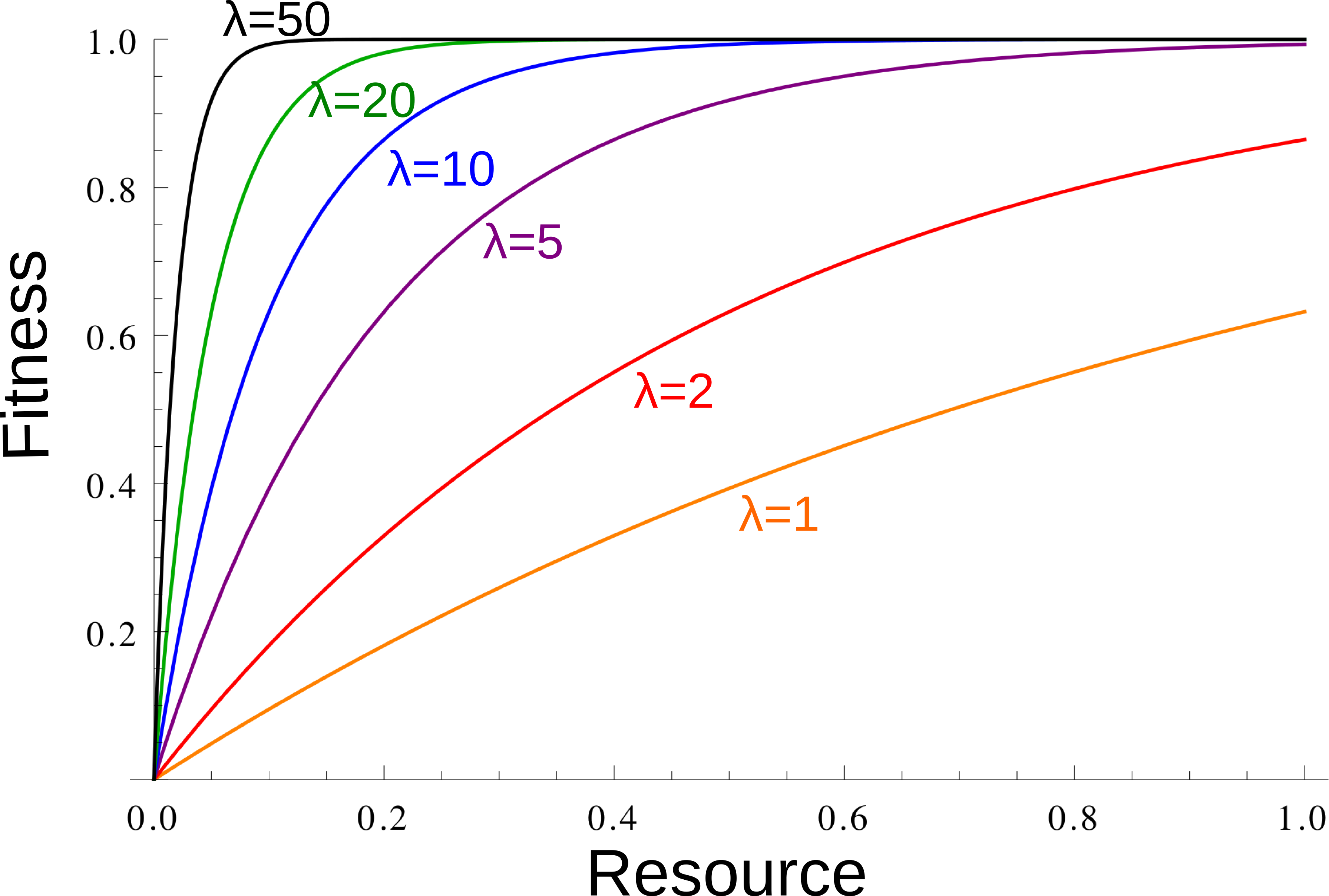
Mean fitness (large dot) for an average resource value (blue), and as the average fitness of two extreme resource
values (red), for a small and a medium \(\lambda\). When \(\lambda\) is larger
(at least for these relatively small value of \(\lambda\)),
average fitness is larger when there is less year-to-year variation, which promotes redistribution: 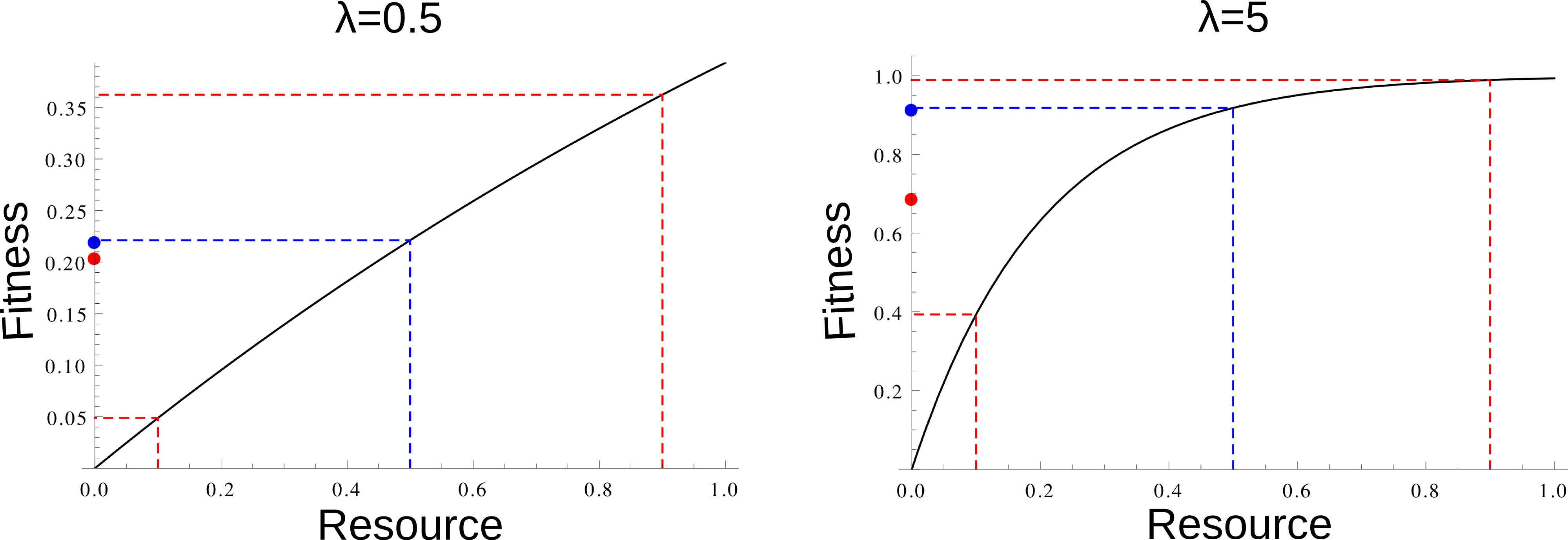
# "sigma" characterize the width of the resource distribution.
The larger sigma, the larger the year-to-year variation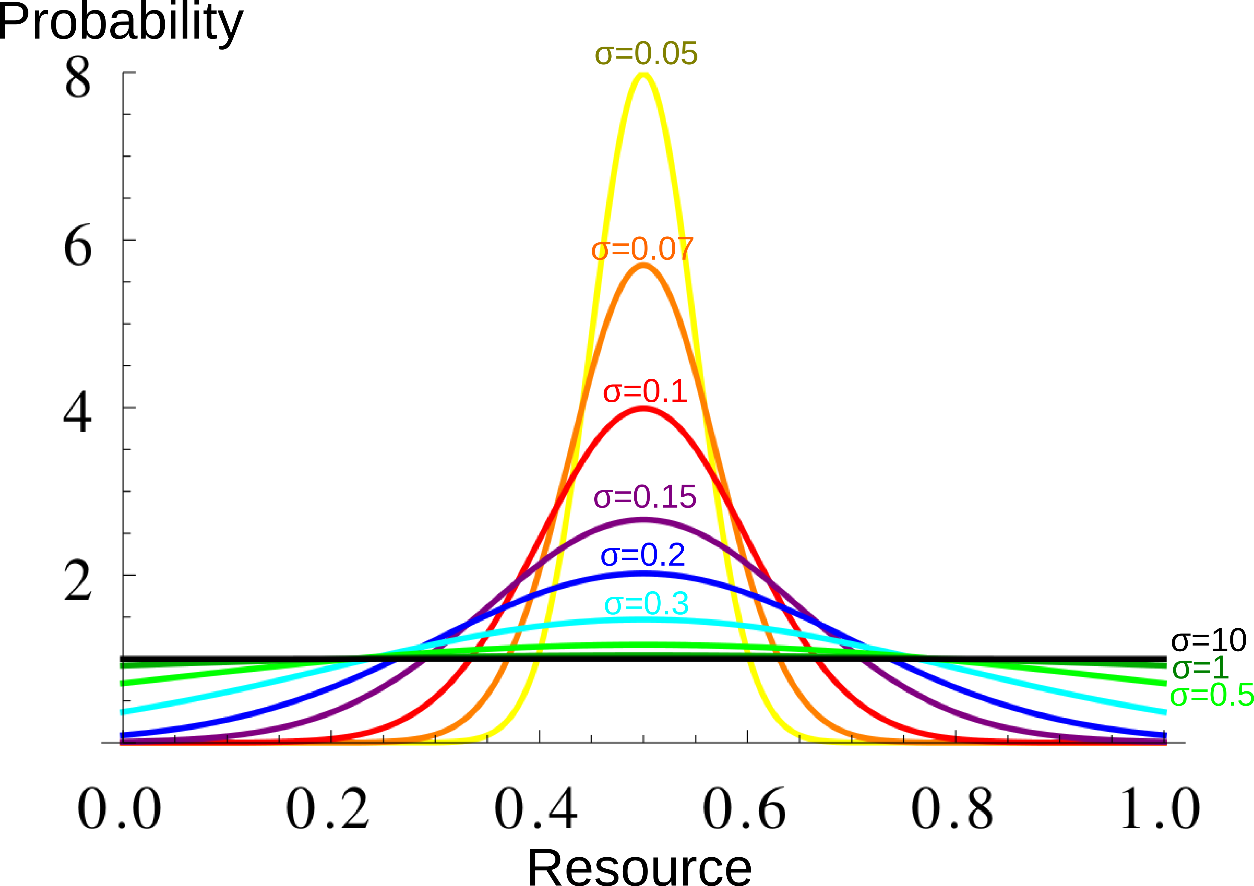
Resource distribution for different \(\sigma\) values. Each year, each individual resource production is taken from this distribution. The larger \(\sigma\), the greater the year-to-year variation.
 slist=c(0.05,0.07,0.1,0.15,0.2,0.3,0.5,1,10) #list of values of sigma for which the simulation is run.

nann=30 # number of cycles, i.e. "years" at which the simulation ends.

kit=100 #  for each set of parameters, how many simulations are run (in general, quantities shown are
# averages over the results from these simulations)
#(for each set of lambda, sigma in  "llist"" and "slist", "kit"" simulations are performed).

napergen=30 # every "year" (i.e: one cycle of the simulation), any individual has a probability 1/napergen of "dying",
# which means being replaced by a copy of another individual. The reproducing individual is chosen at random from
# the population, with probabilities proportional to the fitnesses. So the mean duration of an individual "life" is napergen.
Simulating:
restotal=array(NA,dim=c(length(slist),length(llist),7))
# this array will contain the interesting results from the simulations

for (s in slist){

 # In a group with sharing (ip-1)/(np-1), with mean resource r, the mean fitness expected (integrating over the individual resource distribution) is
  # \int_0^\infty \frac{1}{\sigma \sqrt{2 \pi }Erf(1/(2 \sigma \sqrt{2}))} \exp\left(-\frac{(u-0.5)^2}{ 2 \sigma^2}\right) \left(1 - \exp(-\lambda ((1 - p) u + p r)) \right)
  # which is equal to :
  # 1 + \frac{1}{2 Erf(1/(2 \sigma \sqrt{2}))} \exp\left(\frac{\lambda}{2} (-1+p-2p-2pr+\lambda (1-p)^2\sigma^2)\right) \left(Erf\left(\frac{-1+2\lambda(-1+p) \sigma^2}{2s\sqrt{2}}\right) -   Erf\left(\frac{1+2\lambda(-1+p) \sigma^2}{2s\sqrt{2}}\right) \right)
  # as this function is difficult to calculate numerically, we used another program (mathematica) to obtain tables of values

  #Needed files can be found at www.normalesup.org/~viciana/nocomit5_files/
  table.fnint=read.csv(paste0("nocomit5_files/nocomit5_l",l,"_s",100*s,"_np",np,".csv"),
                       header=FALSE)

                       fnint=function(ip,np,r,l){
                         if (ip<np){
                           table.fnint[min(floor((r+1/lr)*lr),lr),ip]
                         } else {
                           1-exp(-l*r)
                         }
                       }


for (l in llist){

respersimu=c()

for (iter in 1:kit){
# initialisation
pop=matrix(0,ncol=4,nrow=npop)
# population matrix
# every individual agent is a line
# every agent has the following characteristics:
# (1) entry cost of group (from 1 to ncout)
# (2) amount of sharing in the group (from 1 to np)
# (3) value of next "harvest": individual productivity in the next cycle or year in the simulation
# (4) fitness

pop[,1]=sample(1:ncout,npop,replace=TRUE)
pop[,2]=sample(1:np,npop,replace=TRUE)
pop[,3]=0.5
pop[,4]=1 # initialization for the first round to work OK. At each round, some individuals "die", and are replaced with copies of other individuals, weighted by the fitness.
#An individual's characteristics are contained in pop[k,] , with k the number of the individual. pop[,1] is the entry cost of group (from 1 to ncout); pop [,2] amount of sharing in the group (from 1 to np); pop [,3] value of each individual productivity in the next cycle; pop[,4] is the list of the fitnesses.

temp.resource=matrix(0.5,ncout,np) # initialization
time.last.extinction=0
  for (j in 1:nann){

    oldpop=pop # oldpop is to keep the parameters of the population of last round

    # New individuals are born, npop/napergen in average
    temp=runif(npop,0,1) # we take npop random numbers. The ones below 1/napergen will be replaced
    nouveaux=temp<(1/napergen)
    pop[nouveaux,]=pop[sample(1:npop,sum(nouveaux),replace=TRUE,
                                       prob=(pmax(0,pop[,4]))/sum(pmax(0,pop[,4]))),]# parents are chosen proportionnally to fitness
    # change the oldpop to update new group memberships
    oldpop[nouveaux,1:2]=pop[nouveaux,1:2]


# what will the "harvest" look like? Values of individual productivity
pop[,3]=runif(npop,0,1)

# now individuals decide whether to switch groups.


    # matrix of expected fitness for a given individual inside a group integrating on its distribution of resources
    temp.resource2=matrix(NA,ncout,np)
    for (icout in 1:ncout){
      for (ip in 1:np){
        temp.resource2[icout,ip]=fnint((ip-1)/(np-1),temp.resource[icout,ip],l)
      }
    }


    # following decision :
# should I stay? Fitness expected now staying in the group + fitness expected in the next na years,
# integrating over the individual resource distribution.
# Should I leave? ( Fitness expected now in the new group - its entry cost) + max ( fitness expected
# for the next na years staying in this new group, integrating over the individual resource distribution; fitness expected in the initial group for the na next years - cost to reenter the initial group)
# depending on which fitness is higher, the individual decides whether to stay, or to leave to the next group

    # do they switch groups?
    tempp=(0:(np-1))/(np-1)
    for (k in 1:npop){
      # first, the resource from the group
      tempf=matrix(rep(tempp,each=ncout),nrow=ncout,ncol=np)*temp.resource
      # second, the resources of the individual, and of l
      tempf=1-exp(-l*(tempf+matrix(rep(1-tempp,each=ncout),nrow=ncout,ncol=np)*pop[k,3]))
      tempfstay=max(c(tempf[pop[k,1],pop[k,2]]+na*fnint((pop[k,2]-1)/(np-1),temp.resource[pop[k,1],pop[k,2]],l),
                    tempf[pop[k,1],pop[k,2]]+na*temp.resource2-matrix(rep(coutmax*(0:(ncout-1))/(ncout-1),np),nrow=ncout,ncol=np)),
                    na.rm=TRUE)
      # expected fitness this term, cost to move, max of come back vs. staying there
      tempf=tempf-matrix(rep(coutmax*(0:(ncout-1))/(ncout-1),np),nrow=ncout,ncol=np)+
        na*pmax(temp.resource2,
                fnint((pop[k,2]-1)/(np-1),temp.resource[pop[k,1],pop[k,2]],l)-coutmax*(pop[k,1]-1)/(ncout-1)/na)
      if (tempfstay<max(tempf,na.rm=TRUE)) { # moving to another group is better
        if (length(which(tempf==max(tempf,na.rm=TRUE)))==1) {
          pop[k,1:2]=which(tempf==max(tempf,na.rm=TRUE),arr.ind=TRUE)} else {
            tempn=sample(1:length(which(tempf==max(tempf,na.rm=TRUE))),1)
            pop[k,1:2]=which(tempf==max(tempf,na.rm=TRUE),arr.ind=TRUE)[tempn,]
          }
      } # if switching groups is better. No change if staying is better.
    } # on all individuals


    # We can calculate now the actual amount of resource produced in the group this "year" or cycle of the simulation
     temp.dead=sum(is.na(temp.resource)) # let's keep track of the number of dead groups
    temp.resource=matrix(NA,ncout,np)
    for (icout in 1:ncout){
      for (ip in 1:np){
        temp.resource[icout,ip]=mean(pop[(pop[,1]==icout)&(pop[,2]==ip),3])
      }
    }
    if (sum(is.na(temp.resource))>temp.dead){
      time.last.extinction=j
    }
# and now, the fitness
    for (k in 1:npop){
      tempp=(pop[k,2]-1)/(np-1)
      pop[k,4]=1-exp(-l*(temp.resource[pop[k,1],pop[k,2]]*tempp+(1-tempp)*pop[k,3]))
      if (sum(pop[k,1:2]!=oldpop[k,1:2])>0){ # if there was a change, cost to pay
        pop[k,4]=pop[k,4]-(pop[k,1]-1)*coutmax/(ncout-1)
      }
    }

  }# for each year (j)


respersimu=rbind(respersimu,
                 c(sum(!is.na(temp.resource[2:ncout,]))>0, # still costly groups?
                   ((mean(pop[pop[,1]==1,2])-1)/(np-1)),  # mean sharing, no cost groups
                   ((mean(pop[pop[,1]>1,2])-1)/(np-1)), # mean sharing, costly groups
                   sum(!is.na(temp.resource[1,])), # number of surviving no cost groups
                   sum(!is.na(temp.resource[2:ncout,])),# number of surviving costly groups
                   NA,
                   time.last.extinction)) # time of last extinction
}# for each iteration (iter)

restotal[which(s==slist),which(l==llist),] = c(mean(respersimu[,1]),# proportion costly groups?
                 mean(respersimu[,2],na.rm=TRUE),# mean sharing, no cost groups
                 mean(respersimu[,3],na.rm=TRUE),# mean sharing, cost groups
                 mean(respersimu[,4]),#mean number surviving no cost groups
                 mean(respersimu[,5]),# mean number surviving costly groups
                 mean(respersimu[respersimu[,1]==1,5]),# mean number surviving groups, when they survive
                 mean(respersimu[,7])) # man time of last group extinction
}# for each l

}# for each s
Let’s plot the main figure:
tempb=c(-1,5,15,25,35,45,55,65,75,85,95,105)/100
image(log10(slist),llist,restotal[,,1],xlab="s",ylab="l",breaks=tempb,col=rev(heat.colors(length(tempb)-1)),xlim=c(-1.3,1))
contour(log10(slist),llist,restotal[,,3],add=TRUE,levels=c(0.2,0.4,0.6,0.8))
contour(log10(slist),llist,restotal[,,2],add=TRUE,levels=c(0.15,0.25),lty=2)