Jérémie Bettinelli École polytechnique Laboratoire d'informatique (LIX) 91128 Palaiseau Cedex FRANCE E-mail: firstname « . » lastname « at » normalesup « . » org Office: 2023 Phone: (+33) (0)1 77 57 80 61

This page is dedicated to some computer simulations realized with MATLAB. You may click the frames to enlarge their content.

Well-labeled trees

Via the Schaeffer bijection, planar maps are coded by well-labeled trees. They consist in plane trees whose vertices carry integer labels, varying from -1, 0, or 1 along any edge. Their study yields results on scaling limits for random maps.

The following pictures and film clips show some well-labeled trees. The vertical axis gives the vertices height; one of the horizoontal axis gives the labels; the scale of the second horizontal axis is not linear. The number n above is the number of half-edges in the tree (thus equals twice the number of edges).

n = 100

		n = 25 000

		n = 50 000

The following views are "profile shots." The tree structure is not visible. Only the range of values taken by the labels at any height is to be seen. The last frames for n = 100 000 and n = 100 000 already displayed such views.

	n = 110 000	n = 1 000 000

Contour pair

There is a naturel way to encode well-labeled trees by a pair of functions. We clockwise wander along the border of the tree, visiting every one of its vertices (possibly more than once). The first function records the height of the visited vertex, and the second one records its label. We may then recover the well-labeled tree thanks to these two functions. Once we renormalize the time by n, the heights by n^1/2, and the labels by n^1/4, a classical result shows that this pair of functions converges in distribution, for the uniform topology, toward the normalized Brownian excursion and the head of the Brownian snake.

The following pictures display this pair of functions: in red on the top, the height function, and in purple on the bottom, the label function.

	n = 110 000	n = 1 000 000

The Brownian snake

Instead of only considering the label of the vertex we are visiting, we may take into account the labels of the entire ancestral lineage of the visited vertex. This gives us a family of paths. The path corresponding to a vertex has length the height of the considered vertex, and it varies from -1, 0, or 1 each step. This object converges in distribution toward the Brownian snake introduced by Le Gall. We may recover the head of the Brownian snake simply by keeping only the final value of every path. It is also possible to fully reconstruct the snake only from its head.

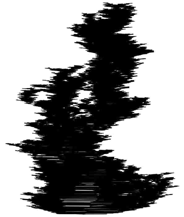
The following picture shows a discrete snake. The shadowy part represents the height function of the associated tree, and we observe a path by cutting the surface at the right depth and by looking at the edge of the cut piece.

n = 100

The following pictures display a Brownian snake approximation. The shadowy part represents the normalized Brownian excursion, and we observe a path by cutting the surface at the right depth and by looking at the edge of the cut piece. The frame on the left allows better to perceive the relief, whereas the frame on the right better shows the "fluffy" feature of the object.